NSA Modules and Branches

A closer look at token compression, selection, gating, and branch mechanisms in NSA

In this section, we cover:

• Token compression
• Token selection and importance scoring
• Sliding window/local context attention
• Gating and branch integration

3.1 Token Compression Module (Section 3.1)

The Token Compression module implements a coarse-grained reduction of the sequence by aggregating tokens into blocks and representing each block with a single compression token (⇒) (⇒). In practice, the sequence of keys (and similarly values) up to the current position $t$ is divided into contiguous blocks of length $l$, with a stride $d$ between block start positions (typically $d < l$ for overlapping blocks) (⇒) (⇒). A learnable function $\phi$ (a small MLP with a positional encoding for the block) compresses each block into one vector, effectively summarizing that block’s information (⇒). Formally, if $k_{1:t}$ denotes the sequence of key vectors from 1 to $t$, the compressed keys at step $t$ are:

$$\tilde{K}^{\text{cmp}}_t \;=\; f^{\text{cmp}}_K(k_{1:t}) \;=\; \Big[\,\phi\big(k_{(i-1)d+1 : (i-1)d + l}\big)\,\Big]_{i=1}^{\left\lfloor\frac{t-l}{d}\right\rfloor}\!,$$

where each $\phi(k_{(i-1)d+1:(i-1)d+l})$ produces a single compressed key for the $i$-th block of length $l$ (⇒) (⇒). Equivalently, the procedure can be described as follows:

• Partition the past keys $k_{1:t}$ into possibly overlapping blocks of length $l$, starting at positions $1, 1+d, 1+2d, \ldots$ (until the end of sequence). Each block covers a segment $k_{j:j+l-1}$ for some starting index $j$. (Typically $d<l$ to ensure blocks overlap and mitigate information fragmentation (⇒).)
• Compress each block into a single vector via a learnable mapping $\phi$. This mapping (an MLP) takes all keys in the block (with an intra-block positional encoding) and outputs one $d_k$-dimensional vector (⇒), which serves as a compressed key representing that entire block. Similarly, a corresponding $f^{\text{cmp}}_V$ produces compressed values $\tilde{V}^{\text{cmp}}_t$ by aggregating each block’s value vectors.
• Collect the compressed keys/values for all blocks. The result $\tilde{K}^{\text{cmp}}_t$ is a set of compressed key vectors, whose number is much smaller than $t$ (approximately $\lfloor (t-l)/d \rfloor$ vectors) (⇒).

This compressed representation captures higher-level, coarser-grained semantics of the sequence while greatly reducing the number of tokens the query has to attend to (⇒). In other words, it provides a global summary of the context with far fewer tokens, which significantly lowers the computational cost of attention on long sequences (⇒). Figure 2 (left) illustrates this branch: the input sequence is processed into compressed attention covering coarse-grained patterns of the sequence (⇒). By using overlapping blocks (if $d<l$), the compression module preserves context continuity between blocks (mitigating hard information cutoffs) at the cost of minor redundancy (⇒). The compressed keys and values from this module (denoted $\tilde{K}^{\text{cmp}}_t, \tilde{V}^{\text{cmp}}_t$) will be used as one branch of the attention mechanism.

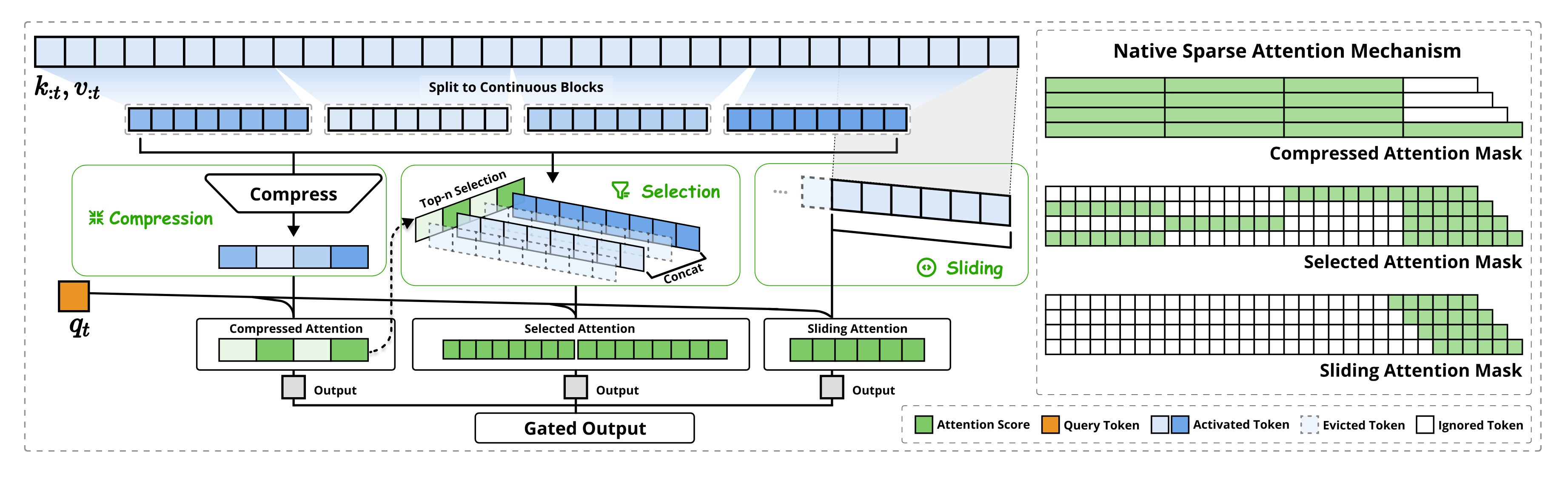
Figure 2, highlighting the Compression branch which groups tokens into coarse blocks and produces one representation per block.

3.2 Token Selection Module – Blockwise Selection (Section 3.2)

The Token Selection module aims to preserve important tokens at full fidelity, complementing the coarse compression branch (⇒). Relying only on compressed tokens could lose critical fine-grained information, so this module selects a subset of original tokens (keys/values) deemed most relevant to the current query. To make this efficient, NSA adopts a blockwise selection strategy – instead of selecting arbitrary individual tokens, it selects contiguous blocks of tokens as units (⇒) (⇒). This strategy is motivated by two considerations:

• Hardware Efficiency: Modern GPU architectures achieve much higher throughput when accessing memory in contiguous blocks rather than scattered indices (⇒). By selecting whole blocks of tokens, the implementation can leverage block-wise memory access and tensor core operations, similar to efficient attention implementations like FlashAttention (⇒). In short, blockwise selection ensures the sparse access pattern remains GPU-friendly and avoids the slowdown of random memory fetches.
• Attention Continuity: Empirically, attention scores tend to exhibit spatial continuity, meaning if one token is important, its neighbors are likely also important (⇒). Prior studies have observed that queries often attend to groups of nearby tokens rather than isolated single tokens (⇒). Thus, selecting an entire block of adjacent tokens (instead of just one) aligns with the natural distribution of attention and is less likely to miss a token that turns out to be important. (Indeed, the authors’ visualization of attention in Section 6.2 confirms this contiguous pattern (⇒).)

Blockwise Selection Implementation: To apply this strategy, the sequence of keys/values is first partitioned into equal-length selection blocks (of length $l'$) (⇒). These blocks are typically non-overlapping contiguous segments of the sequence (for example, block 0 covers tokens $1$ to $l'$, block 1 covers $l'+1$ to $2l'$, and so on). The goal is to identify which of these blocks contain the most relevant tokens for the current query. To do so, NSA computes an importance score for each block (described in Section 3.3 below) and then selects the top-ranking blocks for inclusion in the attention.

Once each block $j$ has been assigned an importance score $p^{\text{slc}}_t[j]$, the selection module chooses the top-$n$ blocks with the highest scores as the active blocks for the query (⇒). Formally, letting $p^{\text{slc}}_t[j]$ be the importance of block $j$, the set of selected block indices is:

$$I_t \;=\; \{\, i \mid \text{rank}\big(p^{\text{slc}}_t[i]\big) \le n \,\} \,, \tag{11}$$

where $\text{rank}(p^{\text{slc}}_t[i])=1$ for the block with highest importance, $\,\le n$ for the top $n$ blocks (⇒). All tokens within those top-$n$ blocks are retained as fine-grained tokens for attention. The keys from the selected blocks are concatenated to form the selected key set $\tilde{K}^{\text{slc}}_t$ for the query (and likewise for values $\tilde{V}^{\text{slc}}_t$) (⇒). This can be written as:

$$\tilde{K}^{\text{slc}}_t \;=\; \text{Concat}\Big\{\,k_{\,i l' + 1 : (i+1) l'} \;\big|\; i \in I_t \,\Big\}\,, \tag{12}$$

meaning $\tilde{K}^{\text{slc}}_t$ is formed by concatenating the original key vectors from each selected block $i$ (⇒). The resulting set $\tilde{K}^{\text{slc}}_t$ has size $n \cdot l'$ (i.e. the module keeps $n$ blocks worth of tokens). An analogous construction produces $\tilde{V}^{\text{slc}}_t$ from the corresponding value vectors (⇒). These selected tokens are then used as a second branch of attention, providing high-resolution information from the most relevant parts of the sequence. In Figure 2 (left), this corresponds to the Selected attention branch, which focuses on “important token blocks” from the input (⇒).

After selection, the keys/values in the chosen blocks are treated just like in standard attention (except limited to those tokens). The attention computation for this branch will operate over $\tilde{K}^{\text{slc}}_t$ and $\tilde{V}^{\text{slc}}_t$, and later be combined with other branches via gating (see Section 3.5). In summary, the token selection module dynamically zooms in on salient regions of the sequence with fine granularity while ignoring less important tokens, all in a hardware-efficient blockwise manner.

Figure 2, highlighting the Selection branch which picks out top-ranked blocks of tokens. The figure shows that only a few blocks (green highlights) are attended, corresponding to important token regions (⇒).

3.3 Importance Score Computation for Token Selection (Section 3.3)

A key challenge in the selection module is scoring the blocks by importance without introducing too much overhead. NSA addresses this by leveraging the computation already done by the compression branch to derive importance scores for free (⇒). The idea is that when the query attends to the compressed tokens, the attention weights on those compressed tokens indicate which portions of the sequence are important. In effect, the compression branch provides a rough importance distribution over the sequence, which can guide the selection branch.

Derivation from Compression Attention: Recall the compression branch yields a set of compressed keys $\tilde{K}^{\text{cmp}}_t$ (one per block of the original sequence). When computing attention for query $q_t$ on these compressed keys, we get a vector of attention scores $p^{\text{cmp}}_t$ corresponding to those blocks. In particular, let $q_t$ be the query vector at position $t$. The attention of $q_t$ over the compressed keys is:

$$p^{\text{cmp}}_t \;=\; \operatorname{Softmax}\!\Big(q_t^\top\,\tilde{K}^{\text{cmp}}_t\Big)\,, \tag{8}$$

which yields $p^{\text{cmp}}_t \in \mathbb{R}^M$ where $M = \big\lfloor\frac{t - l}{d}\big\rfloor$ is the number of compression tokens (blocks) (⇒) (⇒). In other words, $p^{\text{cmp}}_t[i]$ is the normalized attention weight on the $i$-th compressed block for the current query. If $p^{\text{cmp}}_t[i]$ is high, it means the query found block $i$ (covering a certain segment of the sequence) very relevant.

NSA uses $p^{\text{cmp}}_t$ to induce the selection-block importance scores $p^{\text{slc}}_t$. If the selection blocks were chosen to align exactly with the compression blocks (i.e. if the compression block length $l$ equals the selection block size $l'$ and the stride $d$ equals $l$ so there’s a one-to-one correspondence), then we can simply take $p^{\text{slc}}_t = p^{\text{cmp}}_t$ (⇒). In general, the blocking for selection might differ (e.g. $l'$ could be larger or smaller than $l$, or compression blocks might overlap while selection blocks don’t). In that case, each selection block spans one or more compression blocks (or fractions thereof). The importance score for a selection block should then be the aggregate of the compression-based scores for all compression tokens that lie within that selection block’s span (⇒) (⇒). Formally, suppose both $l$ and $l'$ are multiples of the compression stride $d$ (as assumed in the paper). Then the importance of selection block $j$ can be obtained by summing the appropriate entries of $p^{\text{cmp}}_t$ that fall into block $j$’s range:

$$p^{\text{slc}}_t[j] \;=\; \sum_{m=0}^{\frac{l'}{d}-1} \;\sum_{n=0}^{\frac{l}{d}-1} \; p^{\text{cmp}}_t\!\Big(\frac{l'}{d}\,j \;+\; m \;+\; n\Big)\,, \tag{9}$$

which accumulates the softmax weights of all compression tokens whose indices map into selection block $j$ (⇒) (⇒). (This double sum accounts for the possibly overlapping compression blocks within the span of the $j$-th selection block.) In simpler terms, $p^{\text{slc}}_t[j]$ is the total attention mass that the query $q_t$ assigned to the portion of the sequence covered by block $j$ (according to the compression branch’s view).

After computing $p^{\text{slc}}_t$ for every block $j$, the selection module has an importance score for each selection block. These scores are then used to rank the blocks and choose the top $n$ as described in Section 3.2. Because $p^{\text{slc}}_t$ is derived largely from the existing attention computation (the compression branch’s attention), this approach adds minimal computational overhead (⇒). Essentially, NSA recycles the coarse attention results to guide fine-grained token selection.

Multi-Head Considerations: In transformers, multiple attention heads may share the same key-value memory (for example, in grouped-query attention or multi-query attention, several heads use one shared set of keys/values). In such cases, NSA ensures consistent block selection across heads so that all heads in a group pick the same blocks, avoiding redundant memory fetches (⇒) (⇒). They do this by aggregating the importance scores across those heads. If $h=1,\dots,H$ index the heads in a group, the shared importance for block $j$ can be computed as a sum over heads’ importance scores:

$$p'^{\,\text{slc}}_t[j] \;=\; \sum_{h=1}^{H} \;p^{\text{slc},(h)}_t[j]\,, \tag{10}$$

where $p^{\text{slc},(h)}_t$ is the importance vector from head $h$ (⇒) (⇒). The selected blocks are then chosen based on this combined score $p'^{\,\text{slc}}_t$, ensuring all heads in the group attend to the same set of top-$n$ blocks. This synchronization minimizes divergent memory access patterns between heads during decoding (when reading from the key-value cache) (⇒) (⇒).

Summary: The importance score computation module provides the bridge between the compression and selection branches. By computing a query-dependent importance distribution over blocks (using the compression attention output), it enables the token selection module to efficiently pick out the most relevant tokens. These importance scores $p^{\text{slc}}_t$ directly determine which blocks of tokens are fed into the fine-grained selection attention branch (as formalized by Equation (11) in the previous section) (⇒) (⇒). This design preserves crucial information for the query without a heavy computation of its own, thereby maintaining the efficiency of NSA’s sparse attention approach.

3.4 Sliding Window Module for Local Context (Section 3.4)

NSA’s third branch is the Sliding Window module, which explicitly handles local context. This branch ensures that each query always has direct access to the most recent tokens (a fixed-length window of prior tokens), thereby capturing short-range dependencies with high fidelity (⇒) (⇒). The motivation for a dedicated local branch is that local patterns tend to dominate learning in attention networks (⇒). Nearby tokens often have very high relevance (especially in causal language modeling, the immediate past tokens are strong predictors of the next token). If local context is mixed with global context in a single attention, the model may overly focus on these easy-to-use local cues, hindering it from learning long-range patterns (⇒). By isolating local attention in its own branch, NSA allows the model to learn long-range attention in the other branches without being “short-circuited” by always relying on local tokens (⇒) (⇒).

Mechanism: For each query position $t$, the sliding window branch simply takes the last $w$ tokens (keys and values) preceding and including $t$ as the context. These are the tokens in the interval $(t-w, \, t]$ (or [t-w, t] in inclusive indexing) (⇒). Formally, the set of keys and values for the window branch at time $t$ is:

$$\tilde{K}^{\text{win}}_t = k_{\,t-w : t}\,, \qquad \tilde{V}^{\text{win}}_t = v_{\,t-w : t}\,,$$

meaning $\tilde{K}^{\text{win}}_t$ consists of the $w$ most recent key vectors (and similarly for $\tilde{V}^{\text{win}}_t$) (⇒). In practice, $w$ is a fixed window size (e.g. 512 tokens in the authors’ experiments) defining how much immediate context is always attended with full resolution.

This module essentially performs a standard local (sliding-window) attention: the query $q_t$ will attend to the last $w$ keys/values without any sparsification inside this window. What makes it part of NSA’s sparse design is that $w \ll t$ for long sequences, so at any point the query only considers a small local subset in this branch. Crucially, the sliding window branch is separate from the other two branches (compression and selection) (⇒). Its attention output will be combined with the others at the end (via gating), rather than competing directly with them during the attention softmax. This separation means that the presence of strong local correlations does not suppress the learning of long-range attention in the other branches (⇒) (⇒). The authors note that local patterns “adapt faster and can dominate the learning process” if not isolated (⇒), so by giving local context its own branch, other branches can focus on global context without interference (⇒).

Another implementation detail is that NSA uses independent key and value projections for each branch (⇒). In other words, even though the sliding window branch and the global branches might ultimately use some of the same raw tokens (e.g., the most recent tokens could also be part of a compression block or a selected block), the keys/values fed into each branch are obtained from separate learnable transformations. This prevents gradient interference between branches (⇒). For example, the model can adjust the key representations used for long-range compression independently from those used for local window attention. This design choice ensures stable end-to-end training of NSA, as gradients from the local branch (which has a very strong signal) do not distort the representations needed for the global sparse branches (⇒). The overhead of maintaining separate projections is minimal compared to the overall model size, but it greatly helps in preventing one branch from overpowering the others during training (⇒).

In Figure 2 (left), the sliding window module corresponds to the Sliding attention branch that always covers the recent context window for each query (⇒). On the right side of Figure 2, this is visualized as a band along the diagonal of the attention matrix (green squares in a contiguous region near the query token) – indicating that each query attends to its neighboring tokens in the sequence. By including this branch, NSA guarantees that no matter how aggressive the global sparsification (compression/selection) is, the model will not lose track of local context and short-range correlations.

Figure 2 featuring the Sliding Window branch, showing that each query attends to a fixed window of previous tokens. Note how this branch covers the diagonal band of the attention pattern, ensuring local context is attended (⇒).

3.5 Gating and Branch Integration Mechanism (Section 3.5)

NSA combines the outputs of the three parallel branches – compression, selection, and sliding window – using a learned gating mechanism (⇒) (⇒). Rather than simply concatenating or averaging the branch outputs, NSA computes a weighted sum where the weight (gate) for each branch is dynamically determined by the model for each query. This allows the model to adaptively emphasize or de-emphasize each source of information (coarse global context, selected important tokens, or local window) depending on the needs of the current token.

Mathematically, let $o^{cmp}_t = \text{Attn}(q_t, \tilde{K}^{cmp}_t, \tilde{V}^{cmp}_t)$ be the attention output from the compression branch alone (i.e. attending $q_t$ to compressed tokens), and similarly $o^{slc}_t$ from the selection branch and $o^{win}_t$ from the sliding window branch. The gated output $o^*_t$ is given by a sum over branches $c \in \{\text{cmp}, \text{slc}, \text{win}\}$, each scaled by a gate coefficient $g^c_t$:

$$o^*_t \;=\; \sum_{c \in \{\text{cmp},\,\text{slc},\,\text{win}\}} \; g^c_t \;\cdot\; \text{Attn}(q_t,\, \tilde{K}^c_t,\, \tilde{V}^c_t)\,. \tag{5}$$

Here $g^c_t \in [0,1]$ is the gate score for branch $c$ at query $t$ (⇒) (⇒). These gating values are produced by a small neural network (an MLP with a sigmoid activation) that takes as input the query’s features (e.g. the transformer's hidden state or $q_t$ itself) (⇒). Intuitively, $g^c_t$ tells the model how much attention to pay to branch $c$ for this token. For example, if $g^{win}_t$ is high (close to 1) and $g^{cmp}_t$ is low (near 0), then the model is relying mostly on local context for token $t$ and largely ignoring the compressed global context for that token. The gating values are continuous, so the model can blend branches or even use all three if needed (they are not a mutually-exclusive softmax; each gate is independently in [0,1]) (⇒). In practice, the model will learn to set these gates in a way that optimally combines the information sources for each scenario.

The gating mechanism thus performs a learned fusion of the branch outputs. As illustrated in Figure 2 (left), after computing attention in each branch, NSA produces a Gated Output by weighting each branch’s output and summing them (⇒) (⇒). This gating not only merges the information but also can serve to selectively activate branches: if a gate value is near 0, that branch’s contribution is negligible for that token. (For instance, in a situation where the local context provides all necessary information, the model might gate down the other two branches for efficiency.) Because gating is learned end-to-end, the model can flexibly adjust the importance of global vs. local context for different tokens or tasks.

To maintain the efficiency of the sparse attention, the total number of keys/values that the query actually attends to remains low. In fact, the total effective key set size is $N_t = |\tilde{K}^{cmp}_t| + |\tilde{K}^{slc}_t| + |\tilde{K}^{win}_t|$ (⇒). By design of the previous modules, each of these sets is much smaller than $t$, so $N_t \ll t$ even though we have three branches (⇒). This $N_t$ is the sum of compressed tokens, selected tokens, and window tokens considered at step $t$ (see Equation (6) in the paper) (⇒). NSA keeps $N_t$ low (high sparsity) by appropriate choices of block sizes, $n$ (number of selected blocks), and $w$ (window size), so that the combined attention still operates on a sparse set of context tokens per query. In summary, the gating mechanism integrates the three sparse attention branches to produce the final attention output $o^*_t$ (which then goes into the transformer’s next layers), while preserving the computational gains of sparsity.

Figure 2 provides an overview of this integration. The left panel shows the three parallel attention branches (Compression, Selection, Sliding Window) processing the input sequence, and a gating module that combines their outputs into the final result (⇒). The right panel visualizes the attention mask patterns for each branch (green indicates attended positions, white indicates skipped) (⇒). The gating ensures that these patterns are fused appropriately: effectively, the final attention for $q_t$ covers coarse global context (from compression), important specific tokens (from selection), and the immediate neighborhood (from the sliding window), with each part weighted by learned gates. This branch integration via gating is one of NSA’s core innovations, enabling it to balance local and global context in a trainable manner.

Figure 2 shows the gating mechanism: an illustration of the gating MLP taking $q_t$ as input and outputting $g^{cmp}_t$, $g^{slc}_t$, $g^{win}_t$, which then weight the branch outputs. The outputs of the three branches are summed to produce the final $o^*_t$ (⇒) (⇒).