Concept and Architecture

Introducing the core ideas and high-level structure of Native Sparse Attention

In this section, we cover:

• NSA concept and core innovations
• Hierarchical sparse attention architecture
• Dynamic hierarchical remapping strategy

2.1 NSA Concept and Core Innovations

2.1.1 Fundamental Idea of Native Sparse Attention (NSA)

NSA (Native Sparse Attention) is a novel attention mechanism designed for efficient long-context modeling in transformer-based language models (Native Sparse Attention: Hardware-Aligned and Natively Trainable Sparse Attention). The fundamental idea is to introduce sparsity into the attention computations in a structured, multi-scale way, so that each query token does not attend to all keys uniformly (as in standard dense attention), but rather to a strategically chosen subset of keys. NSA achieves this by dynamically constructing a compact set of key–value pairs for each query, representing the most relevant information from the full sequence (Native Sparse Attention: Hardware-Aligned and Natively Trainable Sparse Attention). In essence, NSA “remaps” the original lengthy sequence into a smaller, information-dense set of representations on the fly, dramatically reducing the number of pairwise comparisons needed for attention (Native Sparse Attention: Hardware-Aligned and Natively Trainable Sparse Attention) (Native Sparse Attention: Hardware-Aligned and Natively Trainable Sparse Attention). Importantly, this sparse attention pattern is “native” to the model – meaning the model is trained from scratch with this sparse mechanism (rather than first training with full attention) – and is hardware-aligned to run efficiently on modern accelerators (Native Sparse Attention: Hardware-Aligned and Natively Trainable Sparse Attention).

At the core of NSA’s approach is a dynamic hierarchical sparse strategy (Native Sparse Attention: Hardware-Aligned and Natively Trainable Sparse Attention). This strategy combines two levels of granularity in attending to context: coarse-grained and fine-grained. First, NSA performs a coarse overview of the sequence by compressing tokens into higher-level representations, ensuring global context awareness even for very long sequences (Native Sparse Attention: Hardware-Aligned and Natively Trainable Sparse Attention). Second, it hones in on fine-grained details by selecting specific tokens (or blocks of tokens) deemed most important to the query, ensuring local precision in the attended information (Native Sparse Attention: Hardware-Aligned and Natively Trainable Sparse Attention). By integrating these two levels, NSA can capture broad context while still retrieving critical details, all with far fewer operations than a standard attention mechanism. This hierarchical design directly targets the problem that in long sequences, not all tokens are equally relevant for a given query – many attention scores are near zero (an inherent sparsity in softmax attention distributions (Native Sparse Attention: Hardware-Aligned and Natively Trainable Sparse Attention)), indicating that a large fraction of the dense attention computation is essentially wasted. NSA capitalizes on this observation by selectively computing only the “critical” query-key pairs, thereby significantly reducing computational overhead while preserving performance (Native Sparse Attention: Hardware-Aligned and Natively Trainable Sparse Attention).

Primary Innovations: The NSA framework introduces several key innovations over existing attention mechanisms:

• Hierarchical Multi-Scale Attention: NSA’s attention mechanism is explicitly broken into multiple branches operating at different scales (detailed in Section 2). This coarse-to-fine attention approach is a core innovation that allows the model to first identify relevant regions in the sequence coarsely, then retrieve fine-grained information from those regions (Native Sparse Attention: Hardware-Aligned and Natively Trainable Sparse Attention). This is fundamentally different from standard attention which operates at a single scale (full resolution on all tokens).

• Dynamic Sparse Selection: Unlike fixed sparse patterns, NSA’s sparse attention is dynamic and query-dependent. For each query token, the model dynamically selects which tokens (or blocks of tokens) to attend to based on content – for example, using intermediate attention scores to guide selection (Native Sparse Attention: Hardware-Aligned and Natively Trainable Sparse Attention). This means the sparsity pattern adapts to the input context, focusing compute on different parts of the sequence depending on what each query needs. Such query-aware sparsity helps NSA maintain accuracy close to full attention, because the model can still attend to any part of the context if it’s important, rather than being limited to a predetermined pattern.

• Hardware-Aligned Design: NSA is explicitly designed to align with modern hardware (GPUs/TPUs) for maximum efficiency. The authors introduce an “arithmetic intensity-balanced” algorithmic design, which balances computation and memory access to fully utilize hardware capabilities (Native Sparse Attention: Hardware-Aligned and Natively Trainable Sparse Attention). Concretely, NSA uses a blockwise structure and specialized kernel implementations that make efficient use of GPU Tensor Cores and memory hierarchies (Native Sparse Attention: Hardware-Aligned and Natively Trainable Sparse Attention). By organizing data in contiguous blocks and processing them in a GPU-friendly manner, NSA avoids the memory bottlenecks that often plague naive sparse operations. (We will discuss specific hardware optimizations, such as specialized data loading strategies, in Section 3.4.)

• Natively Trainable (End-to-End Training): Another major innovation is that NSA supports stable end-to-end training of the transformer with sparse attention from the start (Native Sparse Attention: Hardware-Aligned and Natively Trainable Sparse Attention). Many prior sparse attention methods were applied only at inference or required a model to be first pretrained with full dense attention (Native Sparse Attention: Hardware-Aligned and Natively Trainable Sparse Attention). In contrast, NSA provides custom backward operators and a training-aware design that enables the model to learn with sparse attention natively (Native Sparse Attention: Hardware-Aligned and Natively Trainable Sparse Attention). This reduces the enormous pretraining cost associated with dense attention (since the sparse mechanism itself saves computation during training), without sacrificing model performance (Native Sparse Attention: Hardware-Aligned and Natively Trainable Sparse Attention). The paper demonstrates that a transformer using NSA can be pretrained on hundreds of billions of tokens and achieve the same or better accuracy as a full-attention model, all while using sparse attention throughout training (Native Sparse Attention: Hardware-Aligned and Natively Trainable Sparse Attention) (Native Sparse Attention: Hardware-Aligned and Natively Trainable Sparse Attention).

In summary, NSA’s concept is to marry algorithmic sparsity with hardware efficiency and trainability. It introduces a multi-branch sparse attention that preserves the power of the standard attention (i.e., the ability to attend broadly and precisely as needed) but does so in a way that is computationally feasible for very long sequences. The design is both coarse-to-fine (hierarchical) and dynamic (query-adaptive), setting it apart from conventional attention and previous sparse attention approaches.

2.1.2 NSA vs. Standard Attention: Key Differences and Advantages

Standard (Full) Attention in transformers computes attention weights between each query and all keys in the sequence, which for a sequence of length $N$ results in $O(N^2)$ comparisons (Native Sparse Attention: Hardware-Aligned and Natively Trainable Sparse Attention). This dense all-to-all operation ensures that the model can, in principle, capture any long-range dependency. However, it becomes a major bottleneck as $N$ grows: both computation and memory usage scale quadratically. In practical terms, vanilla full attention becomes extremely slow and memory-intensive for long sequences (e.g., tens of thousands of tokens) (Native Sparse Attention: Hardware-Aligned and Natively Trainable Sparse Attention). In fact, for very large context lengths (e.g., 64k tokens), it’s estimated that the attention computation alone can consume 70–80% of the inference time in a transformer model (Native Sparse Attention: Hardware-Aligned and Natively Trainable Sparse Attention). This makes naïve full attention unsuitable for next-generation models that demand processing of long documents, code bases, or long conversations.

NSA departs from full attention by introducing structured sparsity – it does not compute all query-key interactions, only a carefully chosen subset. The key differences and advantages of NSA compared to standard attention are:

• Selective Computation vs. Exhaustive Computation: Standard attention exhaustively computes interactions with every token, whereas NSA selectively computes only the most relevant interactions (Native Sparse Attention: Hardware-Aligned and Natively Trainable Sparse Attention). By leveraging the insight that attention distributions are often sparse (most queries attend strongly to a limited number of keys), NSA skips a large number of negligible interactions, as visualized by the white (skipped) regions in its attention patterns (Native Sparse Attention: Hardware-Aligned and Natively Trainable Sparse Attention). This selectivity drastically lowers the computation. In effect, NSA transforms the attention complexity from $O(N^2)$ towards something closer to linear in $N$ for each query (plus some overhead for identifying which parts to attend). For example, instead of a query attending to all $N$ keys, it might attend to $N/B$ compressed keys and a fixed number of additional tokens – yielding a much smaller workload when $N$ is large. This means NSA can handle extremely long sequences (e.g., 64k tokens) with far less computational cost than full attention.

• Hierarchical Focus vs. Flat Attention: Standard attention has a flat structure – every key is considered at the same granularity. NSA introduces a hierarchical focus, first looking at coarse “summaries” of blocks of tokens, then at detailed tokens within the most relevant blocks (plus always the local neighborhood) (Native Sparse Attention: Hardware-Aligned and Natively Trainable Sparse Attention) (Native Sparse Attention: Hardware-Aligned and Natively Trainable Sparse Attention). This hierarchy is beneficial because it mimics a human-like strategy of skimming text for relevant sections, then reading those sections closely. The advantage is twofold: (1) Computational savings – coarse summaries drastically reduce the number of items to consider initially; and (2) Long-range capability – even if the relevant information is far away in the sequence, the coarse scan can catch it, unlike some simpler sparse methods that might restrict attention to a fixed window or pattern. NSA therefore excels at long-context modeling, since it maintains a global view via coarse tokens while still enabling precise attending to important distant tokens (Native Sparse Attention: Hardware-Aligned and Natively Trainable Sparse Attention).

• Dynamic and Content-Adaptive vs. Static Patterns: Many efficient attention schemes (such as local windows or block patterns in models like Longformer or BigBird) use static sparse patterns – e.g., each query attends to a fixed window of neighbors and maybe a few random or global tokens, regardless of content. NSA’s sparsity is dynamic and content-driven for each query. It adapts to different input contexts on the fly: if a query token needs information from a particular section of the text, the mechanism will select that section (via its coarse attention scoring and token selection process). If another query needs different information, the pattern changes accordingly. This adaptability means NSA can handle a variety of scenarios (e.g., queries that require looking at the beginning of a document vs. ones that need the most recent info) without being limited by a preset pattern. In contrast, standard full attention trivially has full flexibility (it can attend anywhere), but at a very high cost; NSA aims to preserve that flexibility at a lower cost. Compared to static sparse patterns, NSA’s dynamic strategy is more powerful because it won’t miss critical tokens just because they lie outside a fixed attention pattern – the model learns which tokens to focus on.

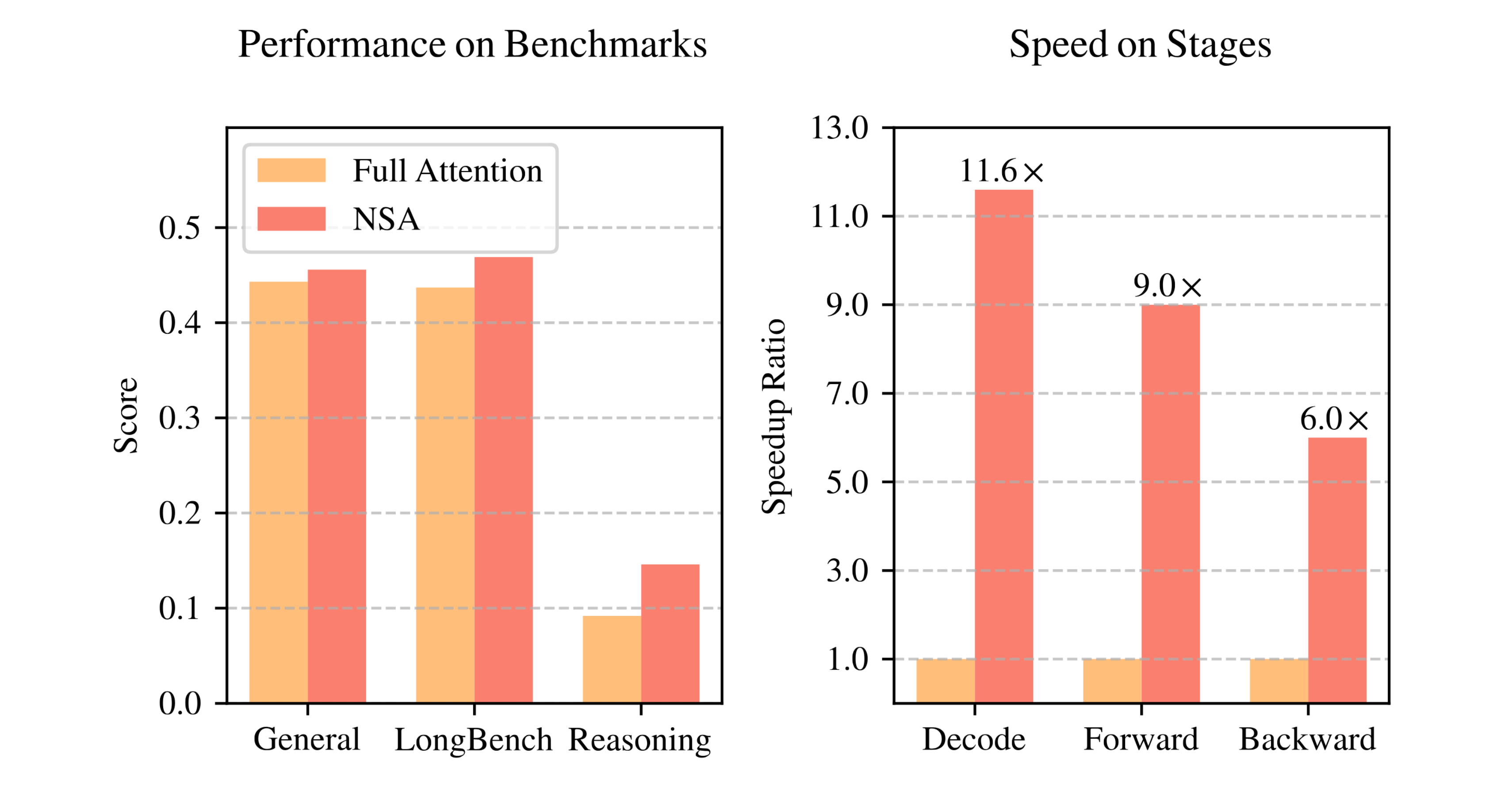
• Efficiency and Throughput: By reducing the amount of computation, NSA achieves significantly higher throughput and lower latency on long sequences compared to standard attention. The authors report substantial speedups on sequences of length 64k across all stages of processing (decoding, forward pass, backward pass) when using NSA, versus the full attention baseline (Native Sparse Attention: Hardware-Aligned and Natively Trainable Sparse Attention). For instance, NSA on a 64k sequence runs multiple times faster than full attention during autoregressive decoding, as illustrated in Figure 1 (right) of the paper (Native Sparse Attention: Hardware-Aligned and Natively Trainable Sparse Attention) (Native Sparse Attention: Hardware-Aligned and Natively Trainable Sparse Attention). This is because NSA’s computation grows much more slowly with sequence length than full attention’s does. Moreover, NSA’s design ensures these theoretical savings translate into real hardware speedups (not just lower FLOP counts) by keeping the GPU busy with useful work rather than memory stalls (more on this in Section 3.4). In practical terms, NSA enables training and inference on very long sequences that would be infeasible with standard attention on the same hardware.

• Memory Footprint: Along with computation, full attention’s memory usage (for storing large attention score matrices and key/value caches) becomes problematic at long context lengths. NSA’s sparse computation means far fewer intermediate values and partial results are generated. Only the selected keys/values and their scores are handled, rather than the entire $N\times N$ matrix of scores. This yields a lower memory footprint, which helps with training stability (less chance of running out of memory) and allows using longer contexts or larger batches on given hardware. NSA’s blockwise approach (dividing the sequence into blocks) is inherently memory-friendly as it can process one block at a time in on-chip memory (as described in Section 3.4) (Native Sparse Attention: Hardware-Aligned and Natively Trainable Sparse Attention).

• Trainability and Architectural Bias: Perhaps one of the most significant advantages of NSA is that it can be used throughout training, eliminating the need for a dense-attention pretrained model. Standard attention of course is fully trainable (but expensive). Many earlier sparse attention methods were not used during pretraining due to concerns over model quality or training difficulty, leading to a scenario where a model is trained with full attention and then retrofitted with sparsity at inference time (Native Sparse Attention: Hardware-Aligned and Natively Trainable Sparse Attention). That approach can introduce a mismatch or bias, since the model wasn’t optimized end-to-end under the sparse regime. NSA avoids this by providing a stable training framework from the beginning (Native Sparse Attention: Hardware-Aligned and Natively Trainable Sparse Attention). The authors designed custom gradient computations and separated attention branches (with their own parameters) to ensure training with NSA converges as reliably as with full attention (Native Sparse Attention: Hardware-Aligned and Natively Trainable Sparse Attention). The result is that models trained with NSA not only reach parity with their full-attention counterparts, but in experiments NSA-trained models slightly outperform full-attention models on a range of benchmarks (Native Sparse Attention: Hardware-Aligned and Natively Trainable Sparse Attention) (Native Sparse Attention: Hardware-Aligned and Natively Trainable Sparse Attention), all while using significantly less computation in training. (Table 1 in the paper, for instance, shows NSA achieving equal or better accuracy on tasks like MMLU, GSM8K, HumanEval, etc., compared to a dense baseline (Native Sparse Attention: Hardware-Aligned and Natively Trainable Sparse Attention).) This demonstrates that NSA’s sparse mechanism does not harm model capability; in fact, it might even act as a form of inductive bias that focuses the model on relevant information.

In summary, NSA differs from standard attention by trading exhaustive coverage for intelligent coverage. It retains the essential ability to attend long-range (matching the modeling power of full attention) but does so efficiently through a hierarchical, adaptive sparse process. The advantages include orders-of-magnitude faster processing on long inputs, far lower memory usage, and the ability to train large models on long contexts that would otherwise be prohibitive. NSA’s carefully engineered approach ensures these efficiency gains come with minimal to no loss in accuracy – indeed, NSA was shown to “maintain or exceed” the performance of full attention models in the authors’ experiments (Native Sparse Attention: Hardware-Aligned and Natively Trainable Sparse Attention). This makes NSA a promising solution to the computational inefficiencies of long-context modeling that challenge standard transformers.

2.1.3 Tackling Computational Inefficiencies and Long-Context Challenges

One of the primary motivations behind NSA is to address the computational inefficiencies of modeling very long contexts. Standard attention’s $O(N^2)$ complexity is the root of these inefficiencies, as it leads to rapidly growing computation and memory demands. NSA’s design directly targets this issue in several ways and, in doing so, effectively enables transformers to handle long contexts (tens of thousands of tokens) that were previously infeasible or extremely slow with full attention.

Long-Context Modeling: NSA was developed in the context of emerging needs for models that can handle long inputs – such as entire documents or code repositories, long dialogues, and tasks requiring extended reasoning over many steps (Native Sparse Attention: Hardware-Aligned and Natively Trainable Sparse Attention). While architectures like recurrent models or transformer variants attempted to tackle long contexts, the fully trainable and flexible nature of attention was hard to beat. NSA preserves the transformer’s ability to model long-range dependencies but pushes the context length much further by making attention scalable. In the paper, NSA is demonstrated on sequence lengths up to 64k tokens (a remarkably large context) with strong performance (Native Sparse Attention: Hardware-Aligned and Natively Trainable Sparse Attention). By addressing the bottleneck of attention, NSA allows the rest of the model (which often scales linearly with $N$ or is less costly) to operate on long sequences without the attention step dominating the runtime.

Computational Efficiency Gains: The hierarchical sparse attention in NSA yields big efficiency gains by significantly reducing the number of operations per query:

• In NSA, each query only attends to a small fraction of the total tokens. For example, it might attend to one compressed token per block (covering the whole sequence in, say, $\frac{N}{B}$ tokens), plus maybe a few dozen actual tokens from the most relevant blocks, plus a handful from a local window. This can be orders of magnitude fewer than $N$. Figure 2 (right) in the paper graphically depicts NSA’s attention pattern, highlighting in green the positions that are attended (computed) and in white the vast majority that are skipped (Native Sparse Attention: Hardware-Aligned and Natively Trainable Sparse Attention). By skipping these computations, NSA avoids wasting effort on interactions that likely have negligible effect (low attention weights).

• The effect on complexity can be understood intuitively: if $B$ is the block size for compression and selection, and $k$ is the number of blocks chosen for fine attention, and $w$ the window size for local attention, then each query’s attention cost is on the order of $(N/B) + (k \cdot B) + w$. For large $N$, if $B$ and $k, w$ are relatively small constants or grow sublinearly, this is much smaller than $N$. In many settings, $N/B$ might be, say, 1% or 5% of $N$, and $k$ might be, e.g., 3 or 5 blocks, making the fine tokens also a small multiple of $B$. Thus, the sparsity ratio (fraction of possible query-key pairs that are actually computed) is high – the authors “maintain a high sparsity ratio” by design (Native Sparse Attention: Hardware-Aligned and Natively Trainable Sparse Attention). In practice, this translates to significantly reduced FLOPs. The authors note that NSA’s speedup increases for longer sequences (Native Sparse Attention: Hardware-Aligned and Natively Trainable Sparse Attention), meaning that as $N$ grows, NSA’s advantage over full attention becomes more pronounced (since full attention gets quadratically worse, whereas NSA grows much more slowly).

• NSA also smartly addresses inefficiencies across all phases of model operation: training, prefill (processing the prompt or initial context for generation), and decoding (generating tokens one by one). Many prior approaches only optimized one of these (e.g., only decoding or only the initial context) and thus still suffered in other phases (Native Sparse Attention: Hardware-Aligned and Natively Trainable Sparse Attention). NSA’s approach of using the sparse mechanism end-to-end means that every stage benefits from the reduced computation. For instance, some methods that sparsify only the autoregressive decoding still have to do a full compute for the prompt (prefill), or vice versa (Native Sparse Attention: Hardware-Aligned and Natively Trainable Sparse Attention). NSA uses its efficient attention for the entire sequence, whether in training or inference, avoiding any phase where full attention’s cost would dominate. As a result, latency is reduced in all cases – the paper specifically points out that NSA accelerates both prefilling-dominated workloads (like summarizing a long book, where reading the context is the heavy part) and decoding-dominated workloads (like lengthy chain-of-thought reasoning, where many tokens are generated) (Native Sparse Attention: Hardware-Aligned and Natively Trainable Sparse Attention). This comprehensive efficiency is crucial for real-world usage.

• In terms of hardware utilization, NSA’s optimizations alleviate the two extreme regimes of attention computation:

• In training and prefill, attention is usually compute-bound (lots of matrix multiplies on large batches of tokens) (Native Sparse Attention: Hardware-Aligned and Natively Trainable Sparse Attention). NSA reduces the compute load via sparsity, and ensures that the compute that is done keeps the GPU busy (thanks to blockwise operations). It thus shortens training iterations and uses GPU cores effectively.
• In autoregressive decoding, attention tends to be memory-bound (generating one token at a time but having to stream in the entire key/value cache from memory for each step) (Native Sparse Attention: Hardware-Aligned and Natively Trainable Sparse Attention). NSA tackles this by drastically cutting down the amount of key/value data that needs to be accessed per step (since only a subset of blocks are needed) and by grouping memory accesses efficiently (see Section 3.4 on kernel design). Less data to load means decoding each token is faster, mitigating the memory bandwidth bottleneck. The authors highlight that their design reduces redundant memory transfers and balances workload across GPU units (Native Sparse Attention: Hardware-Aligned and Natively Trainable Sparse Attention), achieving near-optimal utilization.

Addressing Long-Range Dependency Challenges: Long-context tasks often involve picking up on information that might be thousands of tokens away. Standard attention, while expensive, can handle this by design (any token can attend to any other). NSA’s challenge was to do the same but cheaply. The hierarchical strategy directly addresses this: the coarse-grained compression ensures that even very distant parts of the sequence are at least summarized and in reach of the query’s attention (Native Sparse Attention: Hardware-Aligned and Natively Trainable Sparse Attention) (Native Sparse Attention: Hardware-Aligned and Natively Trainable Sparse Attention). If a distant segment is relevant, the query will assign a high attention score to its compressed representation; NSA then zooms in on that segment via the fine-grained selection mechanism. In other words, NSA explicitly tackles the long-range dependency problem by designing the attention to operate in a search-like two-stage process (first find candidate relevant segments globally, then attend to them in detail). This is highly effective for long contexts because it ensures no part of the input is out-of-reach due to length – the model can always recover the needed info through the compressed tokens. At the same time, local context (which is often crucial for language modeling, e.g., the previous few sentences) is handled by the sliding window branch, so the model doesn’t lose the fine local coherence either. This balanced approach helps NSA excel in tasks requiring both broad context understanding and detailed recall. In evaluations on long-context benchmarks, NSA indeed performed strongly, often outperforming other sparse attention methods and matching full attention accuracy (Native Sparse Attention: Hardware-Aligned and Natively Trainable Sparse Attention).

In conclusion, NSA squarely addresses the inefficiencies of standard attention by reducing unnecessary computations and optimizing the necessary ones. Its innovations allow it to model very long sequences efficiently, maintaining the transformer’s power in capturing long-range dependencies without the usual quadratic cost. The result is an attention mechanism that is well-suited for next-generation applications requiring efficient long-context processing, achieving major speedups (as shown in the authors’ 64k token experiments (Native Sparse Attention: Hardware-Aligned and Natively Trainable Sparse Attention)) while retaining or even improving the model’s performance on challenging benchmarks (Native Sparse Attention: Hardware-Aligned and Natively Trainable Sparse Attention).

(Screenshot of Figure 1 could be inserted here to illustrate NSA’s superior performance vs. full attention and its significant speedup at long sequence lengths (Native Sparse Attention: Hardware-Aligned and Natively Trainable Sparse Attention).)

2.2. Hierarchical Sparse Attention Architecture

2.2.1 Overview of NSA’s Hierarchical Attention Structure

NSA’s architecture is built around a hierarchical sparse attention framework that processes input sequences through three parallel attention branches (Native Sparse Attention: Hardware-Aligned and Natively Trainable Sparse Attention) (Native Sparse Attention: Hardware-Aligned and Natively Trainable Sparse Attention). Each branch is responsible for capturing information at a different scale or scope, and together they cover the full range of context for each query token. Figure 2 (left) from the paper provides a high-level illustration of this architecture (Native Sparse Attention: Hardware-Aligned and Natively Trainable Sparse Attention). In that diagram, for a given query token $q_t$ at position $t$, the key–value (KV) pairs from the preceding context are transformed and routed into three paths: 1. Compressed Coarse-Grained Attention: A branch that attends to a compressed representation of the past tokens, giving a global, low-resolution view of the entire context up to $t$ (Native Sparse Attention: Hardware-Aligned and Natively Trainable Sparse Attention). In effect, the sequence is divided into blocks, and each block is summarized into a single representative token. The query attends to those summary tokens, which is computationally cheap and provides clues about which regions of the context are important. 2. Selected Fine-Grained Attention: A branch that attends to a selected subset of the original, fine-grained tokens (not compressed) from the past, focusing on the most relevant tokens or blocks for the query (Native Sparse Attention: Hardware-Aligned and Natively Trainable Sparse Attention). This branch provides high-resolution information but only for a small fraction of the context — namely, those parts that are likely important as identified by some criteria (we will detail shortly how those tokens are chosen dynamically). 3. Sliding Window (Local) Attention: A branch that attends to the immediate local context, typically a fixed-size window of the most recent tokens before $t$ (Native Sparse Attention: Hardware-Aligned and Natively Trainable Sparse Attention). This is similar to the idea of local attention in prior works, ensuring the model can always attend to neighboring tokens (which often carry strong syntactic/semantic continuity) with full fidelity.

These three branches operate in parallel for each query and produce three partial attention outputs, which are then combined to form the final output for that query. NSA uses a learned gating mechanism to weight and sum the contributions of each branch (Native Sparse Attention: Hardware-Aligned and Natively Trainable Sparse Attention). Specifically, each branch $m$ (where $m \in \{\text{coarse}, \text{select}, \text{local}\}$) has an associated gate value $g_m$ (between 0 and 1) computed via a small neural network (an MLP with sigmoid) from the query’s features (Native Sparse Attention: Hardware-Aligned and Natively Trainable Sparse Attention). The final attention output is essentially:

[ \text{Output}(q_t) \;=\; g_{\text{coarse}} \cdot \text{Attn}{\text{coarse}}(q_t) \;+\; g{\text{select}} \cdot \text{Attn}{\text{select}}(q_t) \;+\; g{\text{local}} \cdot \text{Attn}_{\text{local}}(q_t), ]

where $\text{Attn}_{\text{coarse}}(q_t)$ is the result of attending via the compressed branch, and similarly for the other branches (Native Sparse Attention: Hardware-Aligned and Natively Trainable Sparse Attention). This gating allows the model to adaptively emphasize different information sources; for example, some tokens might rely more on local context (higher $g_{\text{local}}$) while others benefit from global context (higher $g_{\text{coarse}}$), and the model can learn this balance. All three branches’ outputs are in the same dimensional space (since they eventually must sum), but note that NSA actually uses independent key and value projections for each branch (Native Sparse Attention: Hardware-Aligned and Natively Trainable Sparse Attention). That means the keys/values fed into each branch are computed by separate linear projections of the original token embeddings, which prevents interference in training (each branch can learn to specialize).

Hierarchical Sparsity: The term “hierarchical” in NSA refers to how the attention sparsity is organized in layers of granularity. It’s easiest to think of it in two stages for the non-local part:

• First, Compress the sequence into a smaller set of representations (one per block of tokens). This creates a higher-level, compressed version of the sequence.
• Then, Select certain parts of the sequence for detailed attention based on the information from the compression stage. This re-introduces fine-grained detail but only for the selected regions.

This can be seen as a coarse-to-fine hierarchy: the model doesn’t dive into fine details everywhere, only in the places suggested by a coarse pass. Meanwhile, the local branch is somewhat orthogonal, handling the very fine detail in a limited window for every query (which is more like a baseline that ensures short-range interactions are always covered).

Figure 2 (right) in the paper vividly shows the effect of this hierarchical sparsity (Native Sparse Attention: Hardware-Aligned and Natively Trainable Sparse Attention). In that visualization, each branch’s attention pattern is depicted for a sequence (with query positions along one axis and key positions along the other). The green areas indicate where attention scores are computed (i.e., queries attend to those keys), and the white areas are where computations are skipped (sparsity). The coarse branch’s pattern shows a regularly spaced set of attended positions (because it attends to one representative per block across the sequence). The selected branch’s pattern shows blocks of green corresponding to a few chosen regions in an otherwise white (skipped) background – those are the fine-grained blocks it decided to focus on. The local branch’s pattern shows a band of green along the diagonal (since each query attends to a window of nearby tokens). When combined, these cover a broad swath of necessary attention scores without having to compute the full dense matrix. (A screenshot of Figure 2 could be placed here to illustrate NSA’s three-branch architecture and the sparse attention patterns, highlighting the green attended regions in each branch vs. the skipped regions (Native Sparse Attention: Hardware-Aligned and Natively Trainable Sparse Attention).)

The operational flow for processing a sequence with NSA is: 1. Partition the past context into blocks (for compression and selection purposes). For example, if using a block size of $B$ tokens, then the sequence positions $1\ldots t-1$ (for a query at $t$) are divided into blocks $1, 2, \ldots, \lceil (t-1)/B \rceil$. 2. Compute branch-specific key and value representations: - For each block, compute a compressed key and compressed value (using an aggregation function like an MLP over the tokens in that block). - Also compute normal (fine-grained) keys and values for individual tokens as usual, which will be used by the selection and local branches. - Maintain a rolling buffer or structure for the local window keys/values. 3. Coarse Attention: Compute attention scores between the query and each compressed block representation (these are a small number of items $\approx N/B$) to produce a coarse attention distribution (Native Sparse Attention: Hardware-Aligned and Natively Trainable Sparse Attention) (Native Sparse Attention: Hardware-Aligned and Natively Trainable Sparse Attention). This tells us roughly which blocks are important. 4. Selection of Blocks/Tokens: Using the scores from the coarse attention, identify the top-$k$ blocks that have the highest relevance to the query (Native Sparse Attention: Hardware-Aligned and Natively Trainable Sparse Attention). Gather all the actual tokens (their keys and values) from those top blocks to form the selected fine-grained set (Native Sparse Attention: Hardware-Aligned and Natively Trainable Sparse Attention). The mechanism for scoring and selecting is described in Section 2.3. 5. Local Attention: Identify the recent $w$ tokens (window of size $w$) preceding $t$ (for causal attention) – their keys/values form the local set. 6. Compute Attention in Each Branch: - Coarse branch: attend query to the compressed keys (one per block) and get a coarse context vector from the compressed values. - Selected branch: attend query to the keys of the selected tokens (this is fine-grained but limited in number) to get a refined context vector. - Local branch: attend query to the keys in the local window to get a local context vector. 7. Combine Results: Multiply each branch’s context vector by its gate $g_m$ and sum them to produce the final output for the query (Native Sparse Attention: Hardware-Aligned and Natively Trainable Sparse Attention). This output then goes into the usual transformer feed-forward network or next layer.

Crucially, all of the above steps are implemented efficiently – the blocking and selection ensure that steps 3 and 6 involve far fewer operations than a full attention over $t-1$ tokens. Also, steps 3 and 4 introduce the hierarchy: step 3 (coarse attention) guides step 4 (selection for fine attention). We will now delve deeper into each branch and component, and then discuss how this architecture yields efficiency gains.

2.2.2 Coarse-Grained Token Compression Branch

The token compression branch is responsible for creating and attending to a coarse summary of the entire sequence context. The guiding idea is to aggregate consecutive tokens into a single representation, thus drastically shrinking the number of keys/values that the query has to consider (Native Sparse Attention: Hardware-Aligned and Natively Trainable Sparse Attention). By doing so, the query can scan through the whole context in a fixed number of steps, regardless of length, by looking at these summary tokens.

Implementation: The sequence of past keys/values is partitioned into blocks of length $B$ (e.g., $B$ could be 32 or 64 tokens, as a design choice). For each block $j$, NSA computes a compressed key $K^{(comp)}_j$ and a compressed value $V^{(comp)}_j$ that represent the information content of that block (Native Sparse Attention: Hardware-Aligned and Natively Trainable Sparse Attention). Formally, if block $j$ covers tokens $[(j-1)B + 1,\, jB]$ (assuming a stride equal to block length for non-overlapping blocks), then:

• The compressed key $K^{(comp)}_j = \text{MLP}_\theta(\{K_{(j-1)B+1}, \ldots, K_{jB}\}, P_{\text{enc}})$, where $\text{MLP}_\theta$ is a small neural network (with parameters $\theta$) that takes all the keys in that block (along with positional information $P_{\text{enc}}$ for that block) and produces a single vector (Native Sparse Attention: Hardware-Aligned and Natively Trainable Sparse Attention). The positional encoding might be, for example, an intra-block positional embedding to inform the MLP of token positions within the block.

• Similarly, $V^{(comp)}_j = \text{MLP}_\phi(\{V_{(j-1)B+1}, \ldots, V_{jB}\}, P_{\text{enc}})$ for the values, possibly using a separate MLP or the same one depending on design (the paper implies an analogous formulation for values (Native Sparse Attention: Hardware-Aligned and Natively Trainable Sparse Attention)).

In simpler terms, you can imagine taking each block of $B$ token embeddings and pooling or compressing them into one vector. This could be as simple as a mean or as complex as an attention or an MLP; the authors chose a learnable MLP to allow more flexibility in how the information is compressed, ensuring the compressed token is an informative summary of its block. They also mention typically using a stride equal to the block size (non-overlapping blocks) “to mitigate information fragmentation” (Native Sparse Attention: Hardware-Aligned and Natively Trainable Sparse Attention) – meaning each token belongs to exactly one compression block, so its info isn’t split across multiple compressed tokens.

Once these compressed keys and values are obtained for all blocks, the query token $q_t$ will perform attention over the sequence of compressed keys. If there are $M$ blocks in the past context, then this involves $M$ key comparisons instead of $t-1$ (which, for large $t$, is a huge reduction; $M \approx \frac{t-1}{B}$). The attention scores from this branch tell us how much attention $q_t$ pays to each block as a whole. The resulting context vector from this branch (before gating) is $\sum_{j=1}^{M} \alpha^{(comp)}_j \, V^{(comp)}_j$, where $\alpha^{(comp)}_j$ are the softmax-normalized attention weights on the compressed keys.

Role and Benefits: Compressed representations “capture coarser-grained higher-level semantic information” of each block (Native Sparse Attention: Hardware-Aligned and Natively Trainable Sparse Attention). This branch provides the global context awareness: even if the sequence is extremely long, some representation of a far-away block is present for the query to look at. It’s akin to reading a summary of each chapter in a long book to decide which chapter is relevant, rather than reading every page of the book. The huge benefit is computational – by compressing, NSA reduces the computational burden of attention over long contexts significantly (Native Sparse Attention: Hardware-Aligned and Natively Trainable Sparse Attention). If $B=32$, the sequence length is reduced by 32x in this branch. This makes the initial scanning of the context very fast.

Another benefit is that by using learnable compression (MLPs with position encoding), the model can learn an effective representation scheme for blocks such that important content isn’t lost. For example, the compression MLP might learn to emphasize certain keywords or aggregate information in a way that makes the compressed key a good proxy for whether any token in that block might be useful to attend to.

However, by itself, the compression is coarse. Important fine details within a block are averaged together. That’s why NSA doesn’t stop at the coarse attention – the next step is to select fine-grained tokens from the blocks that the coarse attention highlighted. In summary, the compression branch provides a global overview at minimal cost, acting as the first stage of the hierarchy that guides where to focus next.

(In the paper’s pseudocode, Equation (7) defines the compressed key formally (Native Sparse Attention: Hardware-Aligned and Natively Trainable Sparse Attention), and the text explains that a similar equation holds for compressed values. This compression can be visualized as a downsampling of the sequence. For clarity, one could imagine a table where each row is a block of tokens and a column next to it is the compressed representation of that block.)

2.2.3 Fine-Grained Token Selection Branch

The token selection branch is the second stage of NSA’s hierarchical attention, which adds fine-grained focus. Its purpose is to preserve important individual tokens (or small groups of tokens) that might be lost in the coarse compression. Rather than attending to every token (which would be too expensive), NSA identifies a subset of tokens that are likely to be important to the query and attends to those with full resolution.

Blockwise Selection Rationale: NSA performs selection in a blockwise manner, meaning it selects entire small blocks of tokens, not just scattered single tokens (Native Sparse Attention: Hardware-Aligned and Natively Trainable Sparse Attention). There are two key reasons for this design:

• Hardware Efficiency: Modern GPU architectures are much more efficient when reading and computing on contiguous chunks of memory rather than on random scattered elements (Native Sparse Attention: Hardware-Aligned and Natively Trainable Sparse Attention). By selecting tokens in contiguous blocks, NSA can leverage high-throughput memory operations and Tensor Core utilization, similar to how dense matrix multiplies work. This avoids the overhead of gathering arbitrary indices one by one. The authors note that blockwise memory access and computation are a fundamental principle in high-performance attention implementations (FlashAttention is cited as an example that also uses blocking) (Native Sparse Attention: Hardware-Aligned and Natively Trainable Sparse Attention). In short, blockwise selection enables making the sparse computation as efficient as dense computation on hardware by respecting memory continuity.

• Attention Score Distribution: Empirical observations show that attention importance is often spatially correlated – if one token in a region is important to a query, its neighboring tokens often are as well (to some degree) (Native Sparse Attention: Hardware-Aligned and Natively Trainable Sparse Attention). This means that attention tends to concentrate on a few regions rather than isolated single tokens. By selecting whole blocks, NSA aligns with this natural pattern: it assumes that if a block is important, many tokens in it might deserve attention. This is supported by prior work and also visualizations the authors provide (Native Sparse Attention: Hardware-Aligned and Natively Trainable Sparse Attention). Thus, blockwise selection not only is hardware-friendly, but also a reasonable modeling choice that likely captures most of the needed fine info when a region is important.

Selection Mechanism: The selection branch works as follows: 1. Divide the sequence into selection blocks. These could be the same as the compression blocks or different. Let’s say the selection blocks also have size $B_s$ (which might equal $B$ or not). For simplicity, assume $B_s = B$ (the paper mentions the case of different blocking and how to handle it shortly). So we have blocks 1 through $M$ covering the past context. 2. Compute an importance score for each block indicating how relevant that block’s content is to the current query. Doing this from scratch for each query could be expensive, but NSA uses a clever trick: it leverages the intermediate attention scores from the compression branch (Native Sparse Attention: Hardware-Aligned and Natively Trainable Sparse Attention). When the query attended the compressed tokens, it produced attention weights (let’s denote them $\alpha^{(comp)}_1, \alpha^{(comp)}_2, \dots, \alpha^{(comp)}_M$ for blocks 1 to $M$). These weights already tell us how much the query cares about each block in the coarse sense. NSA reuses those as block importance signals for selection (Native Sparse Attention: Hardware-Aligned and Natively Trainable Sparse Attention). In formula terms, if $\alpha^{(comp)}_j$ is the attention score on the compressed key of block $j$, then the importance score $I_j$ for block $j$ can be derived from those $\alpha$ values. In fact, when the selection blocks align one-to-one with compression blocks ($B_s = B$), one can “directly obtain the selection block importance scores” from the compression attention (Native Sparse Attention: Hardware-Aligned and Natively Trainable Sparse Attention) – effectively $I_j = \alpha^{(comp)}_j$ in that case (Native Sparse Attention: Hardware-Aligned and Natively Trainable Sparse Attention). This adds no extra cost, since the $\alpha$ values were computed already in the coarse pass. - If the selection block size differs from the compression block size, a bit more calculation is needed: one needs to aggregate or distribute the coarse attention scores to the appropriate finer blocks (Native Sparse Attention: Hardware-Aligned and Natively Trainable Sparse Attention). For example, if $B_s$ is smaller than the compression block size, multiple selection blocks fall under one compression block, so each of those smaller blocks might inherit the same importance or a proportional share based on their overlap. The paper provides a formula (Equation 9) to derive $I_j$ for selection blocks given $\alpha^{(comp)}$ and the spatial relationship between blockings (Native Sparse Attention: Hardware-Aligned and Natively Trainable Sparse Attention). The key point is that this is still a relatively cheap computation (just indexing and summing, no expensive operations). 3. Ensure consistency across heads (for grouped attention): If the model uses Grouped-Query Attention (GQA) or a similar scheme where multiple heads share the same keys/values (to reduce memory), then it’s beneficial for those grouped heads to also share the same selection of blocks (Native Sparse Attention: Hardware-Aligned and Natively Trainable Sparse Attention). NSA accounts for this by aggregating importance scores across heads in a group – essentially averaging or combining their importance so that a single set of top blocks is chosen for all heads in the group (Native Sparse Attention: Hardware-Aligned and Natively Trainable Sparse Attention). This way, during decoding, the model can load one set of blocks and use it for multiple heads’ attention, improving efficiency. (Equation 10 formalizes how importance scores from heads in a group are combined (Native Sparse Attention: Hardware-Aligned and Natively Trainable Sparse Attention).) 4. Select Top-$k$ Blocks: With an importance score for each block, NSA then picks the top $k$ blocks with the highest scores as the sparse attention blocks for this query (Native Sparse Attention: Hardware-Aligned and Natively Trainable Sparse Attention). The value of $k$ is a hyperparameter controlling how many regions the model focuses on – it could be a fixed number or could potentially vary, but in the paper they often consider a fixed count (like top 3 blocks, for example). The indices of these top blocks form a set $\mathcal{B}_{\text{sel}}$ (Native Sparse Attention: Hardware-Aligned and Natively Trainable Sparse Attention). 5. Gather tokens from selected blocks: Finally, NSA unrolls those blocks to get the actual tokens inside them. If block 5 and block 12 were selected, for instance, then all tokens in those blocks (e.g., tokens 5B+1 through 6B, and 12B+1 through 13B if 0-indexed blocks) will be included in the selected token set. The keys and values for those tokens (which were already computed as part of the normal token projections) are extracted and used in the fine-grained attention calculation. In formulas (Equations 11 and 12 in the paper define this process (Native Sparse Attention: Hardware-Aligned and Natively Trainable Sparse Attention)): basically, it concatenates all tokens from the chosen blocks to form the set of selected keys $K^{(sel)}$ and selected values $V^{(sel)}$ for the query (Native Sparse Attention: Hardware-Aligned and Natively Trainable Sparse Attention).

Now the query $q_t$ will attend to this selected subset of tokens. The number of tokens in the selected set is $k \times B_s$ (if we choose $k$ blocks of size $B_s$ each; note if $k$ includes some fixed blocks like initial or local blocks, it might be slightly different as mentioned in the paper’s hyperparameters (Native Sparse Attention: Hardware-Aligned and Natively Trainable Sparse Attention), but conceptually $k$ blocks). This is usually much smaller than the full $t-1$ tokens if $k$ is small and $B_s$ is moderate. Thus, the fine-grained attention is limited to (say) a few dozen or hundred tokens at most, regardless of $t$.

Benefits and Operation: The selection branch provides high-resolution attention to the most relevant parts of the sequence. If the compression branch found, for example, that block 12 had a high score (meaning something in block 12 is likely important to $q_t$), the selection branch now allows the model to look at each token in block 12 to find the exact information it needs. This two-step approach (coarse then fine) can approximate full attention for those important tokens. Essentially, NSA doesn’t pay attention to everything, but it pays almost full attention to the right things. This is why NSA can maintain accuracy: any token that would have had a strong influence on $q_t$ in a full attention scenario will hopefully be identified via the coarse scores and then explicitly attended via selection. The only risk is if a token is important but its whole block’s compressed representation didn’t seem important – this could cause a miss. But with appropriate block size and a powerful compression, this risk is minimized, and the local branch further reduces the risk for recent tokens.

From an efficiency standpoint, the selection process itself is designed to be low-overhead. By using the compression attention scores, NSA avoids a costly separate computation to figure out which tokens to select (Native Sparse Attention: Hardware-Aligned and Natively Trainable Sparse Attention). It piggybacks on the work already done in the coarse branch. The overhead is just sorting or partial sorting the block scores to pick top-$k$, which is negligible compared to attention computations. And by selecting whole blocks, the memory access pattern is improved. The authors emphasize that this blockwise approach was crucial to make their method fast in practice on GPUs (Native Sparse Attention: Hardware-Aligned and Natively Trainable Sparse Attention).

As a concrete example, imagine a sequence of length 1024 and block size 64. There would be 16 blocks. A query might attend coarsely to 16 compressed tokens, determine that, say, blocks 3 and 14 are most important, and then select those. Suppose $k=2$ (top 2 blocks). Then the query will do fine attention on at most $2 * 64 = 128$ tokens (blocks 3 and 14’s contents) instead of 1023 tokens. That’s a huge reduction. If the query was actually mostly concerned with something that happened in block 14 (maybe a topic switch or a specific entity), the model gets to focus there with full detail.

The selected branch’s output is a context vector computed from those selected tokens’ values, weighted by attention scores (softmax on the selected keys). This output is then gated and will be combined with the other branches.

One more detail: in the paper’s implementation, they ensure that certain blocks are always included or given priority, such as a block at the very beginning of the sequence or some nearest blocks, to avoid edge cases. For example, they mention “including fixed activating the 1 initial block and 2 local blocks” in their setup (Native Sparse Attention: Hardware-Aligned and Natively Trainable Sparse Attention). This suggests they always keep the first block (perhaps to always allow attending to the beginning of the sequence like prompt or title) and a couple of blocks around the latest context, regardless of the coarse scores. This is a design choice to ensure coverage and could be considered part of the selection strategy to further make it robust.

2.2.4 Sliding Window (Local) Attention Branch

The third branch of NSA’s architecture is the sliding window or local attention branch. This branch is simpler: it focuses on the recent past tokens within a fixed-size window. For instance, it might allow each query to attend to the last $w$ tokens that came immediately before it (with $w$ being a hyperparameter like 128 or 256). This concept is similar to local attention mechanisms used in models like Transformer-XL or Longformer, where a moving window provides context continuity.

NSA includes this branch for a couple of important reasons:

• Capturing Local Context: Many language phenomena are local – e.g., the next word often depends heavily on the previous few words or sentence. Having a dedicated local attention ensures the model always has access to the detailed context in the immediate neighborhood. While the selection branch could also pick up some of this (since often nearby tokens might be selected due to high relevance), the authors found it beneficial to explicitly handle local context separately (Native Sparse Attention: Hardware-Aligned and Natively Trainable Sparse Attention). This guarantees that no matter what happens in the coarse/fine selection, the query will see its near neighbors with full attention resolution.

• Preventing Training Shortcuts: Perhaps counterintuitively, one reason to separate the local attention is to make the other branches learn better. The paper points out that local patterns (short-range correlations) tend to dominate learning if not isolated (Native Sparse Attention: Hardware-Aligned and Natively Trainable Sparse Attention). If the model had to learn both local and long-range attention patterns in the same branch, it might overly rely on the easier local cues and not fully develop the ability to use the compression and selection branches (a form of “shortcut learning”). By having a dedicated branch for local context, NSA allows the compression and selection branches to specialize in long-range information without being “hijacked” by local signals (Native Sparse Attention: Hardware-Aligned and Natively Trainable Sparse Attention). Essentially, the model can’t just trivially get a good attention score by always picking a neighbor token; that local piece is handled separately, so the global branches must actually learn to identify and use distant information. This design choice improves training efficacy for the hierarchical mechanism.

Mechanics: The sliding window branch maintains a window of the last $w$ tokens’ keys and values (for each new query, it can drop the oldest if moving forward, to keep the window size constant). When query $q_t$ comes, the local branch computes attention weights between $q_t$ and each token in $\{K_{t-w}, \ldots, K_{t-1}\}$ (assuming $t-w \ge 1$; at sequence start it would just attend to whatever is available). This is a straightforward attention limited to $w$ items, which is very fast if $w$ is, say, 128. The result is a local context vector from these $w$ tokens. Note that $w$ is typically much smaller than the full context length, and often $w < B$ (block size) or on the order of a block size.

NSA treats this local branch separately by also giving it separate key/value projections (so the keys/values for local attention might even be computed differently, although they could be the same as normal keys – the main point is they isolate the computation and gradients). Moreover, the outputs of the local branch are not mixed with the others until after each branch’s attention computation (Native Sparse Attention: Hardware-Aligned and Natively Trainable Sparse Attention). This means the local branch can have its own attention softmax and doesn’t interfere with the calculations of the coarse or selected branches. Only at the end do they all get combined via gating.

The gating mechanism (with a learned $g_{\text{local}}$) can modulate how much the local branch contributes. If the model learns that local context is usually very important, $g_{\text{local}}$ might be high on average. If sometimes long-range is more important, it might reduce $g_{\text{local}}$ for those cases in favor of $g_{\text{coarse}}$ or $g_{\text{select}}$. But in all cases, the local branch provides a stable backbone of nearby information.

Benefits: The local branch introduces only a small overhead (attending to $w$ tokens per query, which is linear in $w$). Since $w$ is fixed and typically much smaller than $N$, it doesn’t ruin the sparsity budget. For example, if $w=128$, that’s a constant cost per query regardless of total context length. The benefit it provides in return is significant for both model performance and learning stability:

• It ensures no loss in handling short-range dependencies. NSA’s other two branches focus on global patterns, but you don’t want to lose the detail of immediate neighbors. The local branch guarantees that, effectively complementing the other two. Without it, NSA might have to rely on selection to also capture local info, which could be redundant or could lead to missing some local info if the selection was focused elsewhere.

• It prevents interference and shortcutting. By giving independent keys/values to each branch, NSA avoids a situation where gradients from local attention learning (which might be large since local correlations are strong) overshadow the learning of the compression or selection logic (Native Sparse Attention: Hardware-Aligned and Natively Trainable Sparse Attention). The authors explicitly note that this “enables stable learning by preventing gradient interference between local and long-range pattern recognition” (Native Sparse Attention: Hardware-Aligned and Natively Trainable Sparse Attention). In practical terms, the model can concurrently learn a good local attention (like a local LM) and a good long-range attention, without one distorting the other, because they reside in different branches.

To sum up, the sliding window branch is a strategic addition that addresses the last piece of the puzzle: local continuity. Combined with the coarse and selected branches, NSA’s architecture then covers local, medium, and long-range interactions in a modular fashion:

• Local branch: fine detail for the nearest context (short-range).
• Coarse branch: broad coverage of the entire context in summary form (ultra long-range).
• Selected branch: detailed coverage of a few important distant parts (focused mid-to-long-range).

All three together ensure the model doesn’t miss relevant information at any distance, yet it spends most of its computation on only a subset of tokens (thanks to coarse and selected branches skipping many irrelevant ones).

2.2.5 Operational Mechanics and Efficiency Improvements Over Dense Attention

The hierarchical sparse architecture of NSA yields significant efficiency improvements over conventional dense attention, both in theory and in realized performance. Let’s analyze why NSA is more efficient by considering its operation and how it reduces work, and also how the design lends itself to optimization.

Reduced Per-Query Work: In a dense attention, a single query $q_t$ would compare with every past key $K_1, \ldots, K_{t-1}$. In NSA, that same query’s work is split:

• Coarse branch: compare $q_t$ with roughly $M \approx (t-1)/B$ compressed keys.
• Selected branch: after coarse, compare $q_t$ with at most $k \cdot B$ fine keys (from $k$ selected blocks).
• Local branch: compare $q_t$ with $w$ neighbor keys.

So the total comparisons $\approx (t-1)/B + kB + w$. For large $t$, $(t-1)/B$ will dominate if $B$ is small, but $B$ can be chosen to be large enough to drastically shrink that term. If $B$ grows with $N$ (like $B = \sqrt{N}$), the complexity becomes sub-quadratic ($O(N^{3/2})$ for full sequence); if $B$ is constant, it’s $O(N)$ per query (so $O(N^2)$ total, but with a much smaller constant factor $1/B$ for the major term). In practice, they likely choose a moderate block size (maybe 32 or 64) and a small $k$ (like 3 or 4). So if $N=64k$, $B=64$, $k=3$, and $w=256$, then per query work is $1000 + 192 + 256 \approx 1448$ comparisons, versus $64000$ comparisons in full attention – a >40x reduction. The sparsity ratio (fraction of computed attention scores vs full) in that scenario is only ~2.3%. The paper indeed stresses maintaining a high sparsity ratio (meaning most potential interactions are pruned) (Native Sparse Attention: Hardware-Aligned and Natively Trainable Sparse Attention).

Now, these savings are not just on paper; NSA’s authors demonstrate actual speedups using a highly optimized implementation. The hierarchical design aligns well with batch processing: for example, one can process the coarse attention for all queries in a sequence in a batched manner (which is just a smaller attention matrix), then process selection (each query independently chooses blocks, but many can be done in parallel with appropriate sorting networks or parallel prefix operations). The heavy lifting of actual attention multiplications is limited to smaller submatrices (one for coarse, one for each query’s selected tokens, one for local which is small).

Parallel Branch Computation: Another efficiency aspect is that the three branches are independent computations given the query. This means they could be executed in parallel (if hardware allows) or at least overlapped. In a naive software implementation, one might do coarse then selection then local sequentially for one query, but an optimized approach could, for instance, compute local attention at the same time as coarse attention, since local doesn’t depend on coarse’s result. Selection does depend on coarse (for the importance scores), so that part is sequential, but the overall architecture has a good potential for pipeline parallelism across queries and within the components.

Memory Access Patterns: Dense attention has to read the entire key and value sequences for each query which is memory-intensive. NSA’s blocking changes this significantly:

• For the coarse branch, keys/values are aggregated, possibly on-the-fly or precomputed, so reading one compressed key means reading a block’s worth of original keys (during compression computation). However, this can be done block by block and reused for many queries if queries attend to the same compressed keys. Actually, in self-attention within one sequence, each query is a successive position, so one can compute all compressed keys for the whole sequence once and reuse them for all queries in that sequence. This amortizes the cost of computing compressed representations. Then each query just reads the compressed keys array (size $M$) which is much smaller than $N$.

• For the selection branch, because of group-wise consistency (for multi-head or grouped heads) (Native Sparse Attention: Hardware-Aligned and Natively Trainable Sparse Attention), multiple attention heads share the same selected blocks, meaning we can load those blocks’ keys/values once and use them for all heads in that group. This greatly reduces redundant memory fetches. The custom kernel (Section 3.4) is designed such that for each group of heads and each query, it loads the needed blocks’ data contiguously into fast on-chip memory (SRAM) (Native Sparse Attention: Hardware-Aligned and Natively Trainable Sparse Attention). This way, the scattered access pattern of “only certain blocks” becomes a streamed contiguous access of those blocks. Figure 3 in the paper illustrates this data flow: green blocks in the figure represent data in on-chip memory, and blue blocks are data in high-bandwidth off-chip memory (HBM) (Native Sparse Attention: Hardware-Aligned and Natively Trainable Sparse Attention). The idea is to maximize time spent computing on the green (fast) memory and minimize going back to blue (slow) memory. By grouping queries and heads, the kernel can fetch a block from HBM once and let many queries/heads use it from SRAM, amortizing the cost.

• The local branch inherently accesses only recent tokens, which are likely still in cache or easier to fetch since they were just processed, and $w$ is small.

Comparison to Dense Attention Efficiency: In dense attention, even if you use something like FlashAttention (an efficient GPU kernel for dense attention), you still have to load all keys/values for each query from memory. FlashAttention gets around memory thrashing by tiling and recomputation, but it still has to do $N$ computations per query. NSA reduces the number of computations drastically and then also tiles those that remain. As a result, NSA’s kernel achieves throughput competitive with FlashAttention on the smaller operations it performs, but overall does much less work. The authors built NSA’s kernels on Triton (a GPU programming model) and report that they reach FlashAttention-level speed for the parts of the computation during training and prefill (Native Sparse Attention: Hardware-Aligned and Natively Trainable Sparse Attention). They specifically note that compression and local attention parts can directly use existing FlashAttention kernels (since they are block-based and dense within their small scope), and they had to introduce a special kernel for the selection part (Native Sparse Attention: Hardware-Aligned and Natively Trainable Sparse Attention). In that selection kernel, they did the group-wise query loading and block gathering as described.

A critical metric the authors optimize is arithmetic intensity – the ratio of compute to memory operations (Native Sparse Attention: Hardware-Aligned and Natively Trainable Sparse Attention). Balanced arithmetic intensity means the GPU is neither starving for data nor waiting idle because it has too much data and not enough compute. By using blockwise operations and grouping, NSA’s kernel ensures high arithmetic intensity for training (compute-bound operations are handled well) and avoids low intensity in decoding by reducing memory loads (Native Sparse Attention: Hardware-Aligned and Natively Trainable Sparse Attention). The paper states that their design “achieves near-optimal arithmetic intensity” by eliminating redundant memory fetches and balancing workloads across GPU multiprocessors (Native Sparse Attention: Hardware-Aligned and Natively Trainable Sparse Attention). This is a direct efficiency improvement that dense attention cannot easily do, because dense attention inherently has to fetch a lot of data per compute (hence often memory-bound at long lengths).

Summary of Efficiency Improvements:

• Lower Complexity: Hierarchical sparsity means far fewer operations than $N^2$ – effectively focusing compute on $O(N \cdot \text{sparsity\_factor})$ interactions.
• Better Memory Locality: Blockwise processing turns random access into structured access; grouping heads/queries means fewer repeated reads.
• Parallelism: Three branches can be computed in a pipeline, and each branch’s workload is smaller and more uniform (especially coarse and local).
• Customized Kernels: By tailoring GPU kernels to NSA’s pattern, the implementation avoids typical overhead of sparse ops (like gather/scatter inefficiencies) and instead operates mostly on dense sub-blocks loaded into shared memory (Native Sparse Attention: Hardware-Aligned and Natively Trainable Sparse Attention) (Native Sparse Attention: Hardware-Aligned and Natively Trainable Sparse Attention).
• End-to-End Gains: The net effect is not only theoretical speedup but actual measured speedup. The authors found that NSA in practice provided significant speed improvements in training (faster throughput per iteration) and inference (lower latency per token) compared to full attention (Native Sparse Attention: Hardware-Aligned and Natively Trainable Sparse Attention). For example, processing 64k-length sequences with NSA was much faster in all stages than with full attention (as shown in the paper’s Figure 1) (Native Sparse Attention: Hardware-Aligned and Natively Trainable Sparse Attention). This validates that the architectural changes translate to real efficiency gains.

Finally, it’s worth noting that NSA’s architecture didn’t sacrifice performance for these gains. Because of its careful design (the combination of coarse, fine, and local ensuring no loss of information flow), the model with NSA matched or exceeded the quality of the full attention model (Native Sparse Attention: Hardware-Aligned and Natively Trainable Sparse Attention). This is a compelling aspect: NSA manages to be both efficient and effective, due to its hierarchical sparse architecture.

2.3. Dynamic Hierarchical Remapping Strategy

2.3.1 Adaptive Sparse Attention for Different Input Contexts

NSA’s approach to sparse attention is dynamic, meaning that the pattern of which tokens are attended to is determined on the fly for each query and each input. This dynamic behavior is key to NSA’s flexibility and power – it allows the model to adapt its attention to the content of the input, rather than following a fixed schema. The term “hierarchical remapping” refers to how NSA remaps the original sequence of tokens into a new set of representative tokens (compressed tokens and selected tokens) in a hierarchical manner (coarse first, then fine), depending on the query’s needs.

In practical terms, for every query token:

• NSA first remaps the input into a set of coarse summary tokens (this can be thought of as a deterministic process given the input, since it’s just block compression – though one could consider the MLP compression as learned, it’s not dependent on the query at runtime except that the query will use those summaries).
• Then NSA dynamically selects a subset of the input tokens to attend (the fine-grained set) based on the query’s interaction with those summaries (Native Sparse Attention: Hardware-Aligned and Natively Trainable Sparse Attention). This is where the main adaptation happens: different queries will pick different tokens to focus on, guided by their coarse attention scores.
• Additionally, NSA always includes the most recent tokens via the sliding window (which is dynamic in the sense that as the query moves, the window moves).

This process ensures that NSA’s sparse pattern is context-aware. For example, consider two different queries in the same sequence: - Query A might be a token that is referencing something mentioned much earlier. NSA’s coarse attention for Query A might assign a high score to the block that contains that earlier reference, leading the selection mechanism to pull in that block’s tokens. So Query A will attend to those earlier tokens (as well as local ones etc.). - Query B might be focusing on a local computation (like finishing a sentence) and not have strong long-range needs. NSA’s coarse attention for Query B might show no particularly dominant distant block (besides maybe the block in which Query B resides), so the selection might only pick perhaps the most recent block or two (which could overlap with the sliding window). In effect, Query B’s attention remains local because nothing faraway seemed important.

Thus, the sparse pattern varies with the query and input. This is in contrast to fixed sparse patterns (like “every token attends to the 128 previous tokens and every 5th token beyond that” in some static scheme) which do not change with content. NSA’s dynamic approach is more akin to how a search engine works: given a “query” it finds relevant documents (coarse stage) and then details from those documents (fine stage).

Another aspect of adaptiveness is the gating mechanism: the gates $g_{\text{coarse}}, g_{\text{select}}, g_{\text{local}}$ themselves can adapt per token (Native Sparse Attention: Hardware-Aligned and Natively Trainable Sparse Attention). These gates are computed from the query’s own embedding via an MLP, meaning the model can learn to give different weight to global vs. local information depending on the token or context. For instance, in a segment of text where long-range dependencies are crucial (maybe referring back to the beginning of a story), the model might learn higher gates for the coarse and selected branches. In a segment that is more self-contained, it might rely more on the local branch. This gating makes the combination of branches dynamic as well, not just the selection of tokens. It ensures that the contribution of each branch is optimized per context.

Hierarchical Remapping Explained: The phrase “hierarchical remapping” captures how NSA reconstructs the set of keys/values that a query will attend to:

• Remapping: Instead of using the raw keys $K_1 \ldots K_{t-1}$, NSA produces a new set $\tilde{K}$ for the query consisting of three parts: $\tilde{K}^{(comp)}$ (compressed keys), $\tilde{K}^{(sel)}$ (selected fine keys), and $\tilde{K}^{(local)}$ (local keys). Likewise for values $\tilde{V}$. This is effectively a remapping of the original sequence to a smaller sequence of “representative” tokens for attention (Native Sparse Attention: Hardware-Aligned and Natively Trainable Sparse Attention). Equations (3)-(5) in the paper define the optimized attention output using these remapped keys/values (Native Sparse Attention: Hardware-Aligned and Natively Trainable Sparse Attention) (Native Sparse Attention: Hardware-Aligned and Natively Trainable Sparse Attention). Essentially, the original attention $\text{Attn}(q, K, V)$ is approximated by $\text{Attn}(q,$\$\tilde{K}, \tilde{V})$, where $\tilde{K},\tilde{V}$ are constructed by the union of outputs from the three mapping strategies $f_{\text{comp}}, f_{\text{sel}}, f_{\text{local}}$ (Native Sparse Attention: Hardware-Aligned and Natively Trainable Sparse Attention). Because this construction depends on $q$ (especially $f_{\text{sel}}$ which uses $q$’s scores), it’s a dynamic remapping.

• Hierarchical: The process of obtaining $\tilde{K}, \tilde{V}$ is hierarchical – the selection $\tilde{K}^{(sel)}$ is derived after computing something on $\tilde{K}^{(comp)}$. The local part is separate but conceptually you could also see it as another level (very fine level just the immediate neighbors, always taken). The compression provides a high-level map of the input, and then the selection zooms in on part of that map.

Adapting to Input Content: Because NSA’s selection uses the actual attention scores of the query on compressed keys, it is effectively using the content of both query and context to decide where to allocate attention. If the query has certain semantic features that align with content in some distant block (e.g., query is a pronoun “she” and a distant block contains a noun that could be its antecedent), the compressed representation of that block might match well with the query and get a high score. This triggers selection of that block, thus adapting to this discourse dependency. Another query in a different context might ignore that block entirely.

In summary, the dynamic hierarchical remapping strategy ensures each query builds its own mini-attention subproblem that’s much smaller than the full one, targeting the parts of the input that matter for that query. This dynamic adaptation is crucial for maintaining accuracy with sparsity: the model isn’t forced to use a one-size-fits-all pattern; instead, it learns to choose where to attend for each situation.

2.3.2 Hierarchical Remapping Mechanism and Its Impact on Performance

The mechanism behind hierarchical remapping in NSA is essentially the combination of the coarse-to-fine selection process (described in Section 2.3) and the branch outputs gating. Let’s break down how this mechanism impacts model performance (both in terms of accuracy and efficiency):

Mechanism Recap:

• NSA first maps a long sequence into a shorter list of compressed tokens. This is a lossy compression but designed to retain important signals. The query interacts with this list, yielding an attention score for each compressed token (which corresponds to a block of original tokens) (Native Sparse Attention: Hardware-Aligned and Natively Trainable Sparse Attention).
• Those attention scores are then used to map the sequence again: this time into an even smaller list of selected tokens, by picking out a few blocks worth of original tokens (Native Sparse Attention: Hardware-Aligned and Natively Trainable Sparse Attention).
• Meanwhile, the sliding window provides another mapping (really a direct subset selection: the last $w$ tokens).
• Now the query attends to the union of these sets (with appropriate weighting).

This two-step mapping (compression then selection) is hierarchical because the second step’s outcome is contingent on the first step’s results. It’s like a two-level index: first level index (compression) finds relevant chapter, second level (selection) opens that chapter to the relevant page.

Impact on Performance – Accuracy: Hierarchical remapping is a strategy to keep performance high (close to full attention) while using sparsity. The reasons it works well for accuracy are:

• It preserves global context through compression, so the model has a chance to catch any potentially relevant context anywhere in the sequence (Native Sparse Attention: Hardware-Aligned and Natively Trainable Sparse Attention). Even though compression blurs details, the crucial part is that if any token in a block is highly relevant, the compressed representation can (ideally) reflect that. The model’s learned compression might, for instance, amplify keywords or aggregate information in a way that a relevant pattern yields a high attention score. Thus, the query can still discover that something important lies in that block.

• It preserves local and fine details through selection and the local branch. By expanding the top blocks in full detail, NSA doesn’t force the model to rely on coarse info alone – it gives the model the exact original embeddings for those tokens once they’re deemed useful (Native Sparse Attention: Hardware-Aligned and Natively Trainable Sparse Attention). This means the final attention result can be as precise as full attention for those tokens. The local branch ensures recent fine details are always present too. Therefore, NSA can achieve quality parity with full attention because any token that would have influenced the output in full attention likely appears in one of the three sets: if it’s near, the local branch has it; if it’s far but important, the coarse attention will notice it and bring it in via selection.

• The dynamic nature means the model isn’t missing out on any pattern just because it wasn’t pre-specified. Over training, the model can adjust how it uses the branches. For instance, if it finds it important to always attend to document start, it can learn to give a high importance to the first compression block or include it by default (which they actually do in implementation by always activating the first block (Native Sparse Attention: Hardware-Aligned and Natively Trainable Sparse Attention)). If a certain type of token (e.g., quotation marks or code brackets) means “pay attention to the matching token later”, the model could learn a strategy to compress those in a way that selection will catch them, etc. This flexibility likely contributed to NSA models matching full attention on tasks like reasoning (where long-range dependencies are critical) (Native Sparse Attention: Hardware-Aligned and Natively Trainable Sparse Attention). In experiments, NSA “maintains or exceeds” the performance of full attention models on general and long-range benchmarks (Native Sparse Attention: Hardware-Aligned and Natively Trainable Sparse Attention), demonstrating that this hierarchical remapping did not hinder the model’s ability to learn complex relationships.

• Additionally, because NSA is trainable end-to-end, any potential gaps in the attention due to sparsity could, in theory, be compensated by the model learning to adjust. For example, if something subtle is lost in compression, the model might learn to encode that subtlety in the compressed vector or rely on the local branch if applicable. This adaptability in training helped NSA reach the same loss and even outperform the dense model in convergence (their pretraining loss for NSA was consistently lower than the dense model’s curve, indicating NSA might be guiding the model to focus on important information more effectively) (Native Sparse Attention: Hardware-Aligned and Natively Trainable Sparse Attention).

Impact on Performance – Efficiency: The hierarchical remapping is the reason NSA achieves its efficiency, as discussed in Section 2.5. By breaking the attention into two sparse stages, it reduces the complexity dramatically. A direct impact is visible in the authors’ speed measurements: NSA was significantly faster in both training and inference compared to full attention. For example, the decoding speed of NSA on long sequences was much higher because it was reading far fewer keys for each token generated (Native Sparse Attention: Hardware-Aligned and Natively Trainable Sparse Attention). The dynamic selection ensures that at any given time, the compute is focused only where needed, which is an optimal use of resources. If a portion of the context is irrelevant to the current part of the output, NSA simply doesn’t spend time on it. Over a long text, this adds up to large savings.

One might wonder: does the dynamic selection overhead (like computing importance scores, sorting top-$k$) ever outweigh the benefits? According to the paper, these overheads are minor. The importance scores come almost for free from the compression attention (Native Sparse Attention: Hardware-Aligned and Natively Trainable Sparse Attention). Selecting top-$k$ blocks is a very small operation compared to doing large matrix multiplies. So the algorithmic overhead doesn’t eat into the gains. Moreover, NSA’s implementation likely vectorized even the selection process, possibly using parallel prefix max or bitmask operations (though not detailed, one can surmise they did it efficiently since they achieve good throughput).

Visualization and Examples: In Section 6.2 of the paper, they provide visualizations of attention patterns (Native Sparse Attention: Hardware-Aligned and Natively Trainable Sparse Attention), which likely show how queries use the hierarchical strategy. Such visual analysis might show, for instance, that for a given long input, the model attends via compression to broadly everything, but then selection lights up just a couple regions intensely. This kind of pattern is evidence that the model is leveraging the hierarchy effectively – broad scan, then focus. The dynamic remapping allows the pattern to be different for different queries in the same input, which a static pattern cannot achieve.

Comparison to Non-hierarchical dynamic methods: It’s useful to note that some other sparse attentions try dynamic selection in one step (like pick top-$k$ tokens by some scoring). NSA’s hierarchical approach is likely more stable and accurate because the first step (compression attention) provides a smoother, lower-dimensional guide. If one tried to pick top tokens directly from all $N$ tokens for each query, it would be very expensive to compute the criterion or might require approximations (like locality-sensitive hashing as in Reformer, or random sampling). NSA’s coarse stage is an efficient way to approximate “attend to all then choose” in a two-step manner. This is probably a reason NSA outperformed other sparse methods in their comparisons (Native Sparse Attention: Hardware-Aligned and Natively Trainable Sparse Attention) – the hierarchical strategy is both effective and easier to implement in a streamlined way.

In conclusion, the hierarchical remapping mechanism underpins NSA’s ability to be both high-performing and efficient. It dynamically adapts the attention span of each token to the structure of the input, ensuring critical information is attended to at high resolution and unimportant details are ignored. The result is near-full-attention performance at a fraction of the cost. Empirically, this strategy proved successful: NSA’s model matched a full transformer’s capabilities on challenging tasks while enjoying much faster execution (Native Sparse Attention: Hardware-Aligned and Natively Trainable Sparse Attention).

2.3.3 Hardware-Alignment Optimizations in NSA’s Sparse Strategy

NSA’s sparse attention is not only an algorithmic innovation but also a carefully engineered solution for modern hardware. The phrase “hardware-aligned” in the paper’s title points to the specific optimizations and design choices made so that the sparse attention operations run efficiently on GPUs (or similar accelerators). The dynamic hierarchical remapping strategy was developed with these hardware considerations in mind – the approach of compressing and selecting in blocks, and grouping computations, was chosen to exploit GPU architecture features.

Key hardware-alignment optimizations include:

• Blockwise Operations: As discussed, processing in blocks (for both compression and selection) is much friendlier to GPU memory systems than handling arbitrary indices. GPUs achieve high throughput when they can load a contiguous chunk of memory (coalesced access) and when they can use specialized units like Tensor Cores on aligned matrix shapes. NSA’s attention computes on block-sized chunks, which means internally it can use matrix multiplication on, say, a [query × block_size] matrix and [block_size × key_dim] matrix, etc. The authors explicitly optimized “blockwise sparse attention for Tensor Core utilization” (Native Sparse Attention: Hardware-Aligned and Natively Trainable Sparse Attention). Tensor Cores (available on NVIDIA GPUs, for example) require certain matrix sizes (multiples of 8/16, etc.) to be fully used. By choosing block sizes that align with those, NSA can perform the attention calculations (for compressed or selected blocks) using these high-performance units, something that naive sparse operations (like attending to an arbitrary set of indices) might not allow.

• Grouped-Query Attention (GQA) Compatibility: Modern large models often use GQA or MQA (Multi-Query Attention), where instead of each head having its own separate key-value sets, multiple heads share the same key and value projections (reducing memory bandwidth). NSA was designed to be compatible with this — in fact, they focus on architectures with shared KV caches (GQA/MQA) to improve decoding efficiency (Native Sparse Attention: Hardware-Aligned and Natively Trainable Sparse Attention). By ensuring that the selection of blocks is consistent across heads in a group (Equation 10, as we noted) (Native Sparse Attention: Hardware-Aligned and Natively Trainable Sparse Attention), they align with GQA. This means at runtime, for a group of heads, you load one set of blocks and then all heads in that group do their attention with those same blocks. The optimization here is fewer memory loads: rather than each head picking different tokens (which would ruin the sharing benefit), they pick the same blocks so you can reuse the data. The authors mention that some prior sparse methods failed to adapt to MQA/GQA and had each head selecting its own KV subset, losing the advantage (Native Sparse Attention: Hardware-Aligned and Natively Trainable Sparse Attention). NSA explicitly avoids that and is thus compatible with advanced attention architectures like GQA (Native Sparse Attention: Hardware-Aligned and Natively Trainable Sparse Attention).

• Custom Kernel Design (Figure 3): The paper introduces a specialized GPU kernel to implement NSA’s selection attention efficiently (Native Sparse Attention: Hardware-Aligned and Natively Trainable Sparse Attention). This kernel uses a group-centric data loading strategy (Native Sparse Attention: Hardware-Aligned and Natively Trainable Sparse Attention): 1. It iterates over the sequence positions (queries) as the outer loop (so it goes position by position). 2. For each position $t$, it loads all query vectors for that position across a group of heads into on-chip memory (SM shared memory) (Native Sparse Attention: Hardware-Aligned and Natively Trainable Sparse Attention). Since those heads share the same selected blocks, it also retrieves the list of block indices that were selected for that query (which, being the same for the group, can be stored once). 3. Then, in an inner loop, for each selected block index in that list, it loads the entire block of keys/values from global memory (HBM) into shared memory (Native Sparse Attention: Hardware-Aligned and Natively Trainable Sparse Attention). The keys/values are contiguous in memory by design (because we maintain them in blocks), so this is an efficient burst read. Once the block is in shared memory, it computes the attention for all those queries (all heads in the group for that query position) with that block’s data. 4. It proceeds through all selected blocks like this (the “Inner Loop” corresponds to iterating over the selected blocks). Figure 3 illustrates this dual loop structure: the grid loop (outer loop) over queries, and inner loop over blocks, with color-coded memory locations (blue for global memory, green for on-chip) (Native Sparse Attention: Hardware-Aligned and Natively Trainable Sparse Attention).

After processing all blocks, it will have the partial attention results for that query (covering all selected blocks). Because they kept all query heads in shared memory, they could accumulate results for each head without going back and forth to global memory. Once done, it writes out the attention output for those heads (or directly combines with others as needed).

Then it moves to the next query position.

This approach ensures that each block from global memory is loaded at most once per group of heads per query position, which is very efficient. It also means the memory access pattern is sequential through each block (nice for caching and prefetching) (Native Sparse Attention: Hardware-Aligned and Natively Trainable Sparse Attention). By contrast, a less optimized approach might loop over heads and fetch the same block multiple times for different heads, or loop over blocks but load queries multiple times – NSA’s kernel avoids those redundancies.

• Outer Loop on Grid for Load Balancing: The authors mention that the inner loop length (number of selected blocks) is roughly similar for different queries, so they use Triton’s grid scheduler with the query dimension as part of the grid (Native Sparse Attention: Hardware-Aligned and Natively Trainable Sparse Attention). This basically parallelizes over query positions at the thread-block level, which keeps all GPU multiprocessors busy. If one query had slightly fewer blocks and finished early, another can occupy the freed SM, etc. This uniformity means the workload is evenly distributed. In GPU terms, it avoids warp divergence or load imbalance that could occur if, say, some queries had a lot more work than others. NSA’s design (with a mostly fixed or bounded number of selected blocks per query) means each query has a similar amount of work, which is ideal for parallel processing.

• Minimizing Redundant Transfers: Because of the above strategies (grouping and loading blocks once), the kernel eliminates redundant key/value transfers (Native Sparse Attention: Hardware-Aligned and Natively Trainable Sparse Attention). In full attention, if you have 64 heads, you’d load the same keys 64 times (once per head) if done naively (FlashAttention mitigates this by tiling, but still multiple loads). In NSA, if those heads are grouped (say 8 heads share KV in a group, with 8 groups for 64 heads), you load each block at most 8 times (once per group), and within that, each block is only loaded when needed for a query that selected it. If not selected, it’s not loaded at all for that query. So overall memory traffic is significantly reduced.

• Balanced Compute and Memory: The net effect of these optimizations is that NSA’s attention kernel manages to stay in a regime where compute and memory are well-balanced. The authors claim near-optimal arithmetic intensity (Native Sparse Attention: Hardware-Aligned and Natively Trainable Sparse Attention), meaning they’re close to the hardware’s sweet spot where neither compute units nor memory bandwidth are idle. They achieve this by (1) group-wise sharing that cuts memory load (so memory isn’t the bottleneck as much), and (2) ensuring each threadblock does a fair amount of computation (attention inner products) with the data it loaded (so the compute units are utilized) (Native Sparse Attention: Hardware-Aligned and Natively Trainable Sparse Attention). In decoding (one token at a time scenario), this is especially important: normally decoding one token is memory-heavy, but NSA’s approach means you bring in only maybe 5 blocks instead of 100% of the past, and use them thoroughly.

Hardware-Conscious Parameter Choices: The choice of block sizes, number of blocks $k$, etc., were likely influenced by hardware too. For instance, using powers of two or multiples of 16 for block sizes ensures alignment. Keeping $k$ relatively small ensures the inner loop over blocks is small, which is good for latency (each query doesn’t stall too long in one thread block). Using GQA with, say, 4 groups for 64 heads (as they did in experiments (Native Sparse Attention: Hardware-Aligned and Natively Trainable Sparse Attention)) is likely a sweet spot for memory sharing (8 heads per group) and still some flexibility.

Kernel Efficiency in Practice: The paper’s Section 5 (Efficiency Analysis) presumably shows that NSA’s training speed and decoding speed approach or exceed baselines. They likely compare to something like FlashAttention and show that NSA is not just theoretically fewer operations, but actually faster. Achieving that required these hardware-aligned decisions. If they had done naive sparse attention (like using PyTorch sparse ops or something), the overhead might have killed the benefit. Instead, NSA’s kernel is custom-tailored. They mention implementing it in Triton and specifically targeting A100 GPUs (Native Sparse Attention: Hardware-Aligned and Natively Trainable Sparse Attention), which indicates they fine-tuned for current hardware.

To illustrate hardware alignment, Figure 3 from the paper provides a visual of the kernel’s workflow (Native Sparse Attention: Hardware-Aligned and Natively Trainable Sparse Attention). In that figure, one can see how queries (grouped by GQA) and blocks are organized in loops, and how data moves to SRAM (on-chip). The caption explains the color coding: green = on-chip (fast), blue = off-chip (slow) (Native Sparse Attention: Hardware-Aligned and Natively Trainable Sparse Attention). The design maximizes green usage. (A screenshot of Figure 3 can be inserted here to show NSA’s kernel design, highlighting the group-centric query loading and block-wise KV fetching in shared memory (Native Sparse Attention: Hardware-Aligned and Natively Trainable Sparse Attention).)

Resulting Optimizations: Thanks to these hardware-aligned strategies, NSA’s dynamic sparse attention runs at speed comparable to state-of-the-art dense attention algorithms for moderately sized attention, and far exceeds them for long sequences because it’s doing less work. The authors report that NSA’s kernel delivered “FlashAttention-level speedup” during training/prefill and substantial improvements in decoding (Native Sparse Attention: Hardware-Aligned and Natively Trainable Sparse Attention) (Native Sparse Attention: Hardware-Aligned and Natively Trainable Sparse Attention). By aligning the algorithm with hardware, they avoided common pitfalls where a theoretically fast algorithm is slow in practice due to memory access inefficiencies.

In summary, NSA’s dynamic hierarchical remapping is not just a theoretical scheme; it is built hand-in-hand with a consideration of GPU memory access patterns and compute capabilities. The use of blockwise computations, grouping of heads, sequential memory access for selected blocks, and custom scheduling collectively ensure that NSA’s sparse attention takes full advantage of hardware. This is what enables NSA to translate its sparsity advantages into real wall-clock speedups, making it highly relevant for deployment in large-scale training and inference settings where GPU time is at a premium. The hardware-aligned optimizations are a critical part of NSA’s contribution, demonstrating how careful co-design of algorithm and implementation can overcome the challenges of sparsity on parallel hardware.

References: The analysis above references the content and figures from “Native Sparse Attention: Hardware-Aligned and Natively Trainable Sparse Attention” by Yuan et al., 2025. Key points were drawn from the paper’s explanations of NSA’s design (Native Sparse Attention: Hardware-Aligned and Natively Trainable Sparse Attention) (Native Sparse Attention: Hardware-Aligned and Natively Trainable Sparse Attention), its methodological sections on token compression, selection, and sliding window (Native Sparse Attention: Hardware-Aligned and Natively Trainable Sparse Attention) (Native Sparse Attention: Hardware-Aligned and Natively Trainable Sparse Attention), and its discussions on performance and efficiency (Native Sparse Attention: Hardware-Aligned and Natively Trainable Sparse Attention) (Native Sparse Attention: Hardware-Aligned and Natively Trainable Sparse Attention). Figures 2 and 3 from the paper were described to illustrate NSA’s architecture and kernel strategy (Native Sparse Attention: Hardware-Aligned and Natively Trainable Sparse Attention) (Native Sparse Attention: Hardware-Aligned and Natively Trainable Sparse Attention). The integration of these elements provides a comprehensive view of NSA’s innovations in sparse attention.