
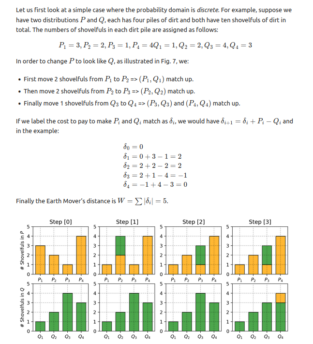
The Wasserstein distance is defined between two probability distributions in order to find the similarity.
- It's equivalently stated as "comparing histograms", as histograms represent distributions.
- Another way of saying this is "a metric on the space of probability measures".
- The Wasserstein distance is also known as the Mallows distance.
A subtype of the Wasserstein distance is the Earth Mover's Distance (EMD), which holds specifically when the two distributions have the same integral (commonly analogised as "two piles with the same amount of dirt").
In economics, it can be used to measure the cost of transportation between two different markets. In ML, it can be used to compare the distributions of data points in different datasets.
Its early applications in the 1980s were in computer vision, since the distribution of pixel values of images are histograms, with EMD you can compare their grayscale brightness intensities (1D) or values in color space (3D).
Levina and Bickel focus on the image processing/computer vision applications, in the late 1990s:
The EMD was first introduced as a purely empirical way to measure texture and color similarities. Rubner et al. demonstrated that it works well for image retrieval.
- Rubner et al. (1998) The Earth Mover’s distance as a metric for image retrieval
Rubner and co's work at Stanford to "describe and summarise different features of an image", sought to compress images themselves and descriptors from signal processing (presumably Fourier etc.) without "quantising" them.
For instance, when considering color, a picture of a desert landscape contains mostly blue pixels in the sky region and yellow-brown pixels in the rest. A finely quantized histogram in this case is highly inefficient. In brief, because histograms are fixed-size structures, they cannot achieve a balance between expressiveness and efficiency.
They proposed variable-size descriptions of distributions or signatures, and the distance between these distributions was the ground distance.
For instance, in the case of color, the ground distance measures dissimilarity between individual colors.
...we capitalize on the old transportation problem (Rachev, 1984; Hitchcock, 1941) from linear optimization, which was first introduced into computer vision by Peleg et al. (1989) to measure the distance between two gray-scale images. ...We give the name of Earth Mover’s Distance (EMD), suggested by [Stolfi][stolfiwiki] (1994), to this metric in this new context.
Kantorovich and Rachev
In 1985 Svetlozar Rachev published The Monge–Kantorovich Mass Transference Problem and Its Stochastic Applications, where he discussed "the Monge optimization problem" (on p.2)
In 1781, Monge formulated the following problem in studying the most efficient way of transporting soil.
Split two equally large volumes into infinitely small particles and then associate them with each other so that the sum of products of these paths of the particles to a volume is least. Along what paths must the particles be transported and what is the smallest transportation cost?
The paper goes on to relate this simple thought experiment to a total of 5 related problems, known as the 'Monge-Kantorovich Problem' (MKP).
Rachev was a doctoral student of Kantorovich, and traces the origin of the EMD to his advisor's work in the 1940s. Between the lines, this talk of "optimal transference" seems to have been motivated by Soviet wartime manoeuvres.
Given two probability measures, the Wasserstein distance is a measure of the "cost" of transforming one measure into the other.
Intuition
This distance measures the amount of "work" required to move one distribution of points to another.
To illustrate with a 1D line (via):
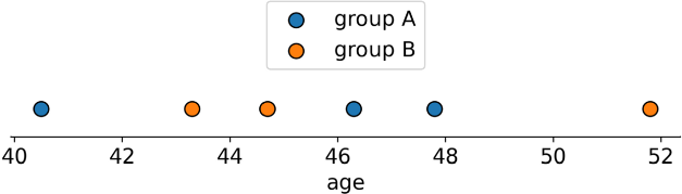
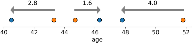
In short: given 2 distributions on a 1D line, it's the average distance you’d have to move each 🔵🟠 pair to reach the nearest while maintaining the relative order (“how hard are they to push together?”)
- The technical term for this is the 'push-forward' operator for discrete measures (Peyré and Cuturi (2018) Computational Optimal Transport)
In other words, it quantifies the difference between two distributions in terms of how much effort would be required to transform one into the other.
Optimal transport
The technique of optimal transport (OT) is said to 'induce' the EMD, as in the paper on Sinkhorn divergences:
a geometric divergence that is relevant to a range of problems. Over the last decade, two relaxations of optimal transport have been studied in depth: unbalanced transport, which is robust to the presence of outliers and can be used when distributions don't have the same total mass; entropy-regularized transport, which is robust to noise and lends itself to fast computations using the Sinkhorn algorithm. This paper combines both lines of work...
It goes on to add:
- OT generalises sorting to spaces of dimension D≥1
- Closely related to minimum cost network flows in optimisation theory
In 2013, Marco Cuturi presented Sinkhorn Distances: Lightspeed Computation of Optimal Transport at NeurIPS
Optimal transportation distances (Villani, 2009, §6) – also known as Earth Mover’s following the seminal work of Rubner et al. (1997) and their application to computer vision – hold a special place among other distances in the probability simplex. Compared to other classic distances or divergences, such as Hellinger, χ2, Kullback-Leibler or Total Variation, they are the only ones to be parameterized This parameter – the ground metric – plays an important role to handle high-dimensional histograms: the ground metric provides a natural way to handle redundant features that are bound to appear in high-dimensional histograms (think synonyms for bags-of-words), in the same way that Mahalanobis distances can correct for statistical correlations between vector coordinates.
Cuturi went on to propose a solution to the high computational complexity of calculating EMD, showing that OT can be regularised by an entropic term, following the maximum-entropy principle, thus making the linear programming problem convex. Its computation can be parallelised and streams well on GPUs.
The paper describes how to compute a 'Sinkhorn distance' using a square cost matrix M of length d
(the data's dimension) and a Lagrange multiplier λ.
Wasserstein is a QQ test
So says the title of section 4.3 of Ramdas et al. (2015) On Wasserstein Two Sample Testing and Related Families of Nonparametric Tests (QQ, or quantile-quantile, plots are used to graphically compare if two datasets came from the same distribution).
Put another way, the Wasserstein distance calculates differences in quantile functions.
Computation
1D Wasserstein
To compute the 1D Wasserstein we can use the SciPy implementation.
from scipy.stats import wasserstein_distance
I initially mistook this for a more general function, but it's documented in the bug tracker:
This is a statistical distance comparing the "distance" between probability measures, since you have the same elements in both arrays I don't see why it should be different than 0
and in another discussion there on a "more general EMD":
Hi everyone, I noticed that the current implementation of the 1d Wasserstein distance (
scipy.stats.wasserstein_distance) is based on '_cdf_distance'. This is fine for now because thel_1Wasserstein distance is equal to the Cramer distance (related to thescipy.stats.energy_distance) but for otherl_pcosts this is not the case.I think it could be a good idea to separate
wasserstein_distancefromenergy_distanceand to clarify the documentation (https://docs.scipy.org/doc/scipy/reference/generated/scipy.stats.wasserstein_distance.html) which is restricted tol_1 Wassersteindistance and which define it as being equal to the Cramer distance. This could be misleading for a naive reader.
Following the link to source
in the docs page
on the SciPy wasserstein_distance function shows it is calculated as the CDF distance between u
and v values (the observed empirical distribution, where u is what moves and v what is moved into).
The _cdf_distance function
(source):
- sorts the values to obtain the 'lexicographical' permutation (the sort ordering).
Let
u_values=[1,2]andv_values=[5,6](i.e. two datasets of two points each, which can be thought of as the original pair moving 4 units upwards along a 1D axis).
u_values, u_weights = _validate_distribution(u_values, u_weights)
v_values, v_weights = _validate_distribution(v_values, v_weights)
u_sorter = np.argsort(u_values)
v_sorter = np.argsort(v_values)
u_values=array([1., 2.])andv_values=array([5., 6.])u_weightsandv_weightsstay asNone(since they're not set).u_sorter=v_sorter=array([0, 1])
- concatenates the unsorted values and sorts them via mergesort (
O(n log n)complexity).
all_values = np.concatenate((u_values, v_values))
all_values.sort(kind='mergesort')
all_values=array([1., 2., 5., 6.])
- Note that this isn't
np.diff(zip(u_values, v_values))! It pairs up values regardless of group.
# Compute the differences between pairs of successive values of u and v.
deltas = np.diff(all_values)
deltas=array([1., 3., 1.])
# Get the respective positions of the values of u and v among the values of
# both distributions.
u_cdf_indices = u_values[u_sorter].searchsorted(all_values[:-1], 'right')
v_cdf_indices = v_values[v_sorter].searchsorted(all_values[:-1], 'right')
u_cdf_indices=array([1, 2, 2])i.e. inserting the first two values of the concatenated list (1,2) on the right hand side of their (identical) values inu(thus1st ,2nd), and the third value (5) after2(thus also2nd).v_cdf_indices=array([0, 0, 1])i.e. inserting the first two values of the concatenated list (1,2) on the left hand side of the values inv(thus both0th), and putting the third value (5) on the right of the (identical) value at position 0 inv(thus1st).
    # Calculate the CDFs of u and v using their weights, if specified.
    if u_weights is None:
        u_cdf = u_cdf_indices / u_values.size
        v_cdf = v_cdf_indices / v_values.size
u_cdf=array([0.5, 1. , 1. ])- monotonic, plateaus at 1v_cdf=array([0. , 0. , 0.5])- monotonic, peaks at 1/2
# Compute the value of the integral based on the CDFs.
# If p = 1 or p = 2, we avoid using np.power, which introduces an overhead
# of about 15%.
if p == 1:
    return np.sum(np.multiply(np.abs(u_cdf - v_cdf), deltas))
u_cdf - v_cdf=array([0.5, 1. , 0.5])this is clearly the distance, and taking theabsof it would make it non-negative (distance not displacement). These pairwise distances then get multiplied by thedeltas(which were paired up consecutively, regardless of group), givingarray([0.5, 1. , 0.5]) * array([1., 3., 1.])=array([0.5, 3. , 0.5]). These products are then simply summed up, giving4.0.
Multidimensional Wasserstein
An example of multi-dimensional histograms was given in the non-bug reported to SciPy above:
distribution1: the animal has a 50% chance to be a cat, 50% to be a dog, 0% tiger, 0% lion;distribution2: the animal has a 0% chance to be a cat, 0% to be a dog, 50% tiger, 50% lion,
As maintainer Pamphile Roy points out,
For it to work with this distance: since you have a 3-dimensional distribution, you have to either assume no correlation and do 3 analyses (and possibly combining them together in a single metric) or you need to work on the 3-dimensional distribution at once (not supported by SciPy).
In the thread on "a more general EMD" Jonathan Vacher suggests the Python Optimal Transport library, POT. POT's intro discusses Wasserstein distances between distributions and goes on to specifically look at how to compute it:
It can be computed... directly with the function
ot.emd2.
# a and b are 1D histograms (sum to 1 and positive)
# M is the ground cost matrix
W = ot.emd2(a, b, M)  # Wasserstein distance / EMD value
The reason for the 2 in the function name is that the library supplies the OT matrix or the computed value, and where the value is produced the name is suffixed with 2.
- See also the API docs for
ot.emd2
To take an example with equal values out of order that Liliang Weng gives in her essay on Wasserstein distances:
- P = [3,2,1,4]
- Q = [1,2,4,3]
- EMD = 5
P = np.array([3,2,1,4]).astype(float)
Q = np.array([1,2,4,3]).astype(float)

# for moving cost from ith index in A to jth index in B
ip = np.arange(0, P.shape[0], 1)
iq = np.arange(0, Q.shape[0], 1)
n = P.shape[0]
M = ot.dist(ip.reshape((n, 1)), iq.reshape((n, 1)), 'euclidean')

W = ot.emd2(P, Q, M)
This indeed gives W to be 5.0.
3D Wasserstein distance
An example of 3D data is given in the docs:
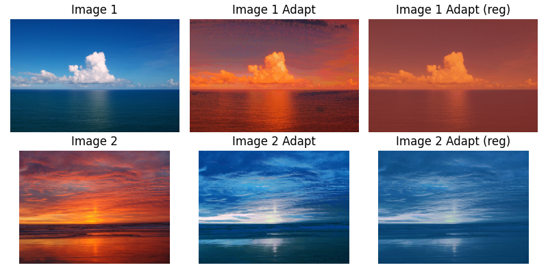
The recipe goes:
- Get some images as
(0,1)normalised float dtype matrices, and reshape them from (h, w, dim) into (h * w, dim) (a 3D vector representing the pixel RGB values). Equivalent to usingreshape(h * w, -1). These are yourX1andX2. - Randomly sample 500 training samples from the source and target (
XsandXt). - Instantiate the transport algorithms:
- EMD:
py ot_emd = ot.da.EMDTransport() ot_emd.fit(Xs=Xs, Xt=Xt) transp_Xs_emd = ot_emd.transform(Xs=X1) transp_Xt_emd = ot_emd.inverse_transform(Xt=X2) - Entropy-regularised EMD:
py
ot_sinkhorn = ot.da.SinkhornTransport(reg_e=1e-1)
ot_sinkhorn.fit(Xs=Xs, Xt=Xt)
transp_Xs_sinkhorn = ot_sinkhorn.transform(Xs=X1)
transp_Xt_sinkhorn = ot_sinkhorn.inverse_transform(Xt=X2)
- EMD:
- Clip the results back between (0,1) and reshape back to the original image shape
As a simple example, consider again some blue pixels becoming red pixels: in fact consider one pixel.
im1 = np.array([[[0,0,1]]]).astype(float)
im2 = np.array([[[1,0,0]]]).astype(float)
These are two square 1x1 RGB images, im1 all blue and im2 all red.
We'd expect their EMD to be high if we indeed calculate it correctly in 3D!
import ot

X1 = im1.reshape(im1.shape[0] * im1.shape[1], -1)
X2 = im2.reshape(im2.shape[0] * im2.shape[1], -1)

rng = np.random.RandomState(42)
n_samples = 4

idx1 = rng.randint(X1.shape[0], size=(n_samples,))
idx2 = rng.randint(X2.shape[0], size=(n_samples,))

Xs = X1[idx1, :]
Xt = X2[idx2, :]

ot_emd = ot.da.EMDTransport()
ot_emd.fit(Xs=Xs, Xt=Xt)

transp_Xs_emd = ot_emd.transform(Xs=X1)
transp_Xt_emd = ot_emd.inverse_transform(Xt=X2)

im1t = np.clip(transp_Xs_emd.reshape(im1.shape), 0, 1)
im2t = np.clip(transp_Xt_emd.reshape(im2.shape), 0, 1)
As expected, the blue im1 was transported to a red im1t,
and the red im2 was transported to a blue im2t.
>>> im1t
array([[[1., 0., 0.]]])
>>> im2t
array([[[0., 0., 1.]]])
Resources
- What is Wasserstein distance? by Lilian Weng (2017)
- Optimal Transport for Imaging and Learning by Gabriel Peyré (2017)
- A gentle intro to method of Lagrange multipliers by Jason Brownlee
- Understanding Lagrange multipliers visually
(YouTube) by Serpentine Integral
- In particular: at 11:58 the Lagrange multiplier
λis shown: it shows that the extrema of a function subject to a cnstraint occurs where their gradients are parallel, which can also be stated as where they are scalar multiples, withλbeing the multiplier.
- In particular: at 11:58 the Lagrange multiplier
- Course notes on OT by Gabriel Peyré (WIP)
- Part 9 (p.40) covers Wasserstein loss functions
Fun things
- VisualStringDistances.jl, a Julia package to compute the 'visual distance' between letters using Sinkhorn divergence computed by unbalanced OT.